Quantity Indices in the Construction of the GDP Series

John M. Hartwick

Economics Department, Queen’s University, Kingston, Canada.

DOI: 10.4236/tel.[phone]                

Abstract

We provide a critique of the use of Fisher’s Ideal Quantity Index in the construction of the GDP series. Attention is focused on an alternative which factors nominal GDP increase into a sum of a quantity index and a price index rather than a product of a quantity index and a price index. A twenty period example is used to compare approaches.

Keywords

Quantity Indices, GDP Time-Path

1. Introduction

When we say “national product rose by ten percent since last year”, we usually mean that

$\frac{V^{t+1}}{V^t}=1.10$

for $V_t=p_1^t{q}_1^t+p_2^t{q}_2^t+\cdots +p_n^t{q}_n^t$ and $V_{t+1}=p_1^{t+1}{q}_1^{t+1}+p_2^{t+1}{q}_2^{t+1}+\cdots +p_n^{t+1}{q}_n^{t+1}$ for $p_i^t$ and $q_i^t$ the price and quantity of commodity i in period t, the base year. The problem with this statement is that we do not know how much of the ten percent increase was due to prices changing and how much quantities changing across consecutive periods. The index number problem here is to separate these two dimensions of change across periods as effectively as we can. With national output we are focused on the change in quantities of commodities and we would like a procedure that “neutralizes” the inevitable price changes from the quantity changes.

2. Index Numbers

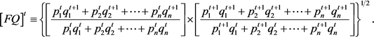
Professional statisticians measure value-change in GDP with the following formula (Fisher’s Ideal Quantity Index ( ${\left[FQ\right]}^t$ )):

(1)

Inside the braces are two familiar index numbers, first a Laspeyres quantity index and secondly a Paasche quantity index. They get multiplied by each other and the product receives a square root operation. ${\left[FQ\right]}^t$ is then a geometric mean of two index values. Observe that each of the two terms in the product has prices the same, top and bottom, while quantities are varying. This formula due to Irving Fisher (1867-1947) is “half” of the following product

$\frac{V^{t+1}}{V^t}={\left[FQ\right]}^t\times {\left[FP\right]}^t$ (2)

where ${\left[FP\right]}^t$, the “other half”, is Fisher’s Ideal Price Index:

${\left[FP\right]}^t={\left\{\left[\frac{p_1^{t+1}{q}_1^t+p_2^{t+1}{q}_2^t+\cdots +p_n^{t+1}{q}_n^t}{p_1^t{q}_1^t+p_2^t{q}_2^t+\cdots +p_n^t{q}_n^t}\right]\times \left[\frac{p_1^{t+1}{q}_1^{t+1}+p_2^{t+1}{q}_2^{t+1}+\cdots +p_n^{t+1}{q}_n^{t+1}}{p_1^t{q}_1^{t+1}+p_2^t{q}_2^{t+1}+\cdots +p_n^t{q}_n^{t+1}}\right]\right\}}^{1/2}.$

Equation (2) says that nominal value-change, $\frac{V^{t+1}}{V^t}$, decomposes mutiplicatively

into a quantity index (itself a geometric mean) and a price index (also a geometric mean). This interesting decomposition¹ has inspired professional statisticians to employ Fisher’s Ideal Quantity Index as the “workhorse” for defining the series of GNP (gross national product). In employing Fisher’s quantity index, statisticians know that there remains another term that is “picking up” the change in prices. Hence ${\left[FQ\right]}^t$ becomes a measure of value-change due to quantities changing, with prices neutralized in a particular way. Price-change effects get left in the price value-change index and are thus taken to be netted out of change in value of national product over two periods. See Table 1 for a multi-period numerical example.

Why should we think that the ${\left[FQ\right]}^t$ index should be the standard for measurement? It has the property: if all prices are multiplied by $\lambda$, the index values will remain unchanged. This is a good price neutrality property. Howerver, one is left with the thought that professional statisticians have come to favor the ${\left[FQ\right]}^t$ index because 1) it makes intuitive sense, 2) it belongs to the attractive

multiplicative decomposition of the nominal $\frac{V^{t+1}}{V^t}$ and 3) it descends from the oeuvre of an economist, prominent in the history of economics.

Current practice for ‘‘constructing’’ real GDP for Canada is reported on in Statistics Canada document 13-107, Section 2.3, ‘‘other aspects of the Income and Expenditure Accounts’’. Fisher’s Ideal Quantity Index is set out and the FQ is linked to actual calculation of real GDP. Current practice is defended there as follows: ‘‘to provide users with a more accurate measure of real growth for GDP

Table 1. A multi-period numerical example

and its components between two consecutive periods and to make the Canadian measure comparable with the National Income and Product Accounts (NIPA) of the United States, which has used the chain Fisher index formula to measure real GDP since 1996’’ (Section 2.136). Diewert (1976) advocates for the use of the Fisher Ideal quantity index ( ${\left[FQ\right]}^t$ ) in Sections 4 and 5 of his well-known article. There is considerable analysis in these sections. Diewert (1978) is favorably cited in Statistics Canada document 13-107, Section 2.3. (‘‘In 1978 Diewert demonstrated that a Fisher index was approximately consistent, and that therefore it was possible to calculate Fisher indexes from aggregates already in Fisher. This solution provides a valid approximation provided that the aggregates used in the calculation are relatively consistent in terms of prices.’’)

3. A Linear Decomposition

Instead of $\frac{V^{t+1}}{V^t}$ being decomposed into the product of price and quantity indices, we consider an additive decomposition: $\frac{V^{t+1}-V^t}{V^t}={\left[HQ\right]}^t+{\left[HP\right]}^t$ with ${\left[HQ\right]}^t$ a quantity index and ${\left[HP\right]}^t$ a price index². We start with a Laspeyres price index, $L^P$. We define $\Delta Q$ in $\frac{V^{t+1}}{V^t}-L^P$, for have then

$\frac{V^{t+1}}{V^t}=L^P+\Delta Q$

for $L^P\equiv \frac{p_1^{t+1}{q}_1^t+p_2^{t+1}{q}_2^t+\cdots +p_n^{t+1}{q}_n^t}{p_1^t{q}_1^t+p_2^t{q}_2^t+\cdots +p_n^t{q}_n^t}$

and $\Delta Q\equiv \frac{p_1^{t+1}\left[q_1^{t+1}-q_1^t\right]+p_2^{t+1}\left[q_2^{t+1}-q_2^t\right]+\cdots +p_n^{t+1}\left[q_n^{t+1}-q_n^t\right]}{p_1^t{q}_1^t+p_2^t{q}_2^t+\cdots +p_n^t{q}_n^t}\mathrm{.}$

This “reads”: nominal GDP percentage increase equals a price change term (a Laspeyres price index) plus a quantity-change term, $\Delta Q$. We can then write a similar identity with first a Laspeyres quantity index, $L^Q$. This defines $\Delta P$.

$\frac{V^{t+1}}{V^t}=L^Q+\Delta P$

for $L^Q\equiv \frac{p_1^t{q}_1^{t+1}+p_2^t{q}_2^{t+1}+\cdots +p_n^t{q}_n^{t+1}}{p_1^t{q}_1^t+p_2^t{q}_2^t+\cdots +p_n^t{q}_n^t}$

and $\Delta P\equiv \frac{q_1^{t+1}\left[p_1^{t+1}-p_1^t\right]+q_2^{t+1}\left[p_2^{t+1}-p_2^t\right]+\cdots +q_n^{t+1}\left[p_n^{t+1}-p_n^t\right]}{p_1^t{q}_1^t+p_2^t{q}_2^t+\cdots +p_n^t{q}_n^t}\mathrm{.}$

We have again a linear decomposition of nominal GDP percentage change, now into a Laspeyres quantity index plus a price-change term.

Since $L^P=1$ for no prices changing between periods, we focus on $L^P-1$. ( $L^P-1$ might be 0.04.) Hence we have

$\frac{V^{t+1}}{V^t}-1=\left\{L^P-1\right\}+\Delta Q\mathrm{.}$

Similar steps we followed above lead to

$\frac{V^{t+1}}{V^t}-1=\left\{L^Q-1\right\}+\Delta P\mathrm{.}$

We proceed to switch $\Delta P$ and $\Delta Q$. Our linear decomposition of $\frac{V^{t+1}-V^t}{V^t}$ is now

$\frac{V^{t+1}-V^t}{V^t}=\frac{1}{2}\left[\left\{L^P-1\right\}+\Delta P\right]+\frac{1}{2}\left[\left\{L^Q-1\right\}+\Delta Q\right]\mathrm{.}$

Our price term in $\frac{V^{t+1}-V^t}{V^t}$ is

$\begin{array}{c}{\left[HP\right]}^t=\frac{1}{2}\left[\left\{L^P-1\right\}+\Delta P\right]\\ =\frac{1}{2}[\frac{q_1^t\left[p_1^{t+1}-p_1^t\right]+q_2^t\left[p_2^{t+1}-p_2^t\right]+\cdots +q_n^t\left[p_n^{t+1}-p_n^t\right]}{p_1^t{q}_1^t+p_2^t{q}_2^t+\cdots +p_n^t{q}_n^t}\\ +\frac{q_1^{t+1}\left[p_1^{t+1}-p_1^t\right]+q_2^{t+1}\left[p_2^{t+1}-p_2^t\right]+\cdots +q_n^{t+1}\left[p_n^{t+1}-p_n^t\right]}{p_1^t{q}_1^t+p_2^t{q}_2^t+\cdots +p_n^t{q}_n^t}]\mathrm{,}\end{array}$ (3)

and the quantity term is

$\begin{array}{c}{\left[HQ\right]}^t=\frac{1}{2}\left[\left\{L^Q-1\right\}+\Delta Q\right]\\ =\frac{1}{2}[\frac{p_1^t\left[q_1^{t+1}-q_1^t\right]+p_2^t\left[q_2^{t+1}-q_2^t\right]+\cdots +p_n^t\left[q_n^{t+1}-q_n^t\right]}{p_1^t{q}_1^t+p_2^t{q}_2^t+\cdots +p_n^t{q}_n^t}\\ +\frac{p_1^{t+1}\left[q_1^{t+1}-q_1^t\right]+p_2^{t+1}\left[q_2^{t+1}-q_2^t\right]+\cdots +p_n^{t+1}\left[q_n^{t+1}-q_n^t\right]}{p_1^t{q}_1^t+p_2^t{q}_2^t+\cdots +p_n^t{q}_n^t}]\mathrm{.}\end{array}$ (4)

We have then a linear decomposition of $\frac{V^{t+1}-V^t}{V^t}$ into price and quantity terms (indices): ( ${\left[HP\right]}^t$ and ${\left[HQ\right]}^t$ ). We can simplify a little. We take 1/2 inside the appropriate square brackets. We then have an arithmetic average of the two prices, $\frac{p_i^t+p_i^{t+1}}{2}={\bar{p}}_i^t$ in one case, and of the two quantities, $\frac{q_i^t+q_i^{t+1}}{2}={\bar{q}}_i^t$ in the other case. This leads to

${\left[HP\right]}^t=\frac{{\bar{q}}_1^t\left[p_1^{t+1}-p_1^t\right]+{\bar{q}}_2^t\left[p_2^{t+1}-p_2^t\right]+\cdots +{\bar{q}}_n^t\left[p_n^{t+1}-p_n^t\right]}{p_1^t{q}_1^t+p_2^t{q}_2^t+\cdots +p_n^t{q}_n^t}$

and ${\left[HQ\right]}^t=\frac{{\bar{p}}_1^t\left[q_1^{t+1}-q_1^t\right]+{\bar{p}}_2^t\left[q_2^{t+1}-q_2^t\right]+\cdots +{\bar{p}}_n^t\left[q_n^{t+1}-q_n^t\right]}{p_1^t{q}_1^t+p_2^t{q}_2^t+\cdots +p_n^t{q}_n^t}.$

Our basic linear decomposition is now the sum of a quantity-change term and a price-change term, across two periods: $\frac{V^{t+1}-V^t}{V^t}={\left[HQ\right]}^t+{\left[HP\right]}^t$. We have

linear averages of quantities and prices in our formulas. We reformulate in terms of percentage price and quantity changes.

$\begin{array}{c}\frac{V^{t+1}-V^t}{V^t}=\frac{p_1^t{\bar{q}}_1^t{P}_1^t+p_2^t{\bar{q}}_2^t{P}_2^t+\cdots +p_n^t{\bar{q}}_n^t{P}_n^t}{p_1^t{q}_1^t+p_2^t{q}_2^t+\cdots +p_n^t{q}_n^t}\\ +\frac{{\bar{p}}_1^t{q}_1^t{Q}_1^t+{\bar{p}}_2^t{q}_2^t{Q}_2^t+\cdots +{\bar{p}}_n^t{q}_n^t{Q}_n^t}{p_1^t{q}_1^t+p_2^t{q}_2^t+\cdots +p_n^t{q}_n^t}\mathrm{.}\end{array}$

for $P_i^t=\left[p_i^{t+1}-p_i^t\right]/p_i^t$ and $Q_i^t=\left[q_i^{t+1}-q_i^t\right]/q_i^t$. Each index is now a weighted sum of percentage changes, with the weights summing to approximately unity. We calculate the quantity index, ${\left[HQ\right]}^t+1$ and place results in the Table. The values for are a small amount above the corresponding values for the Fisher Ideal Quantity Index. It is our opinion that the two series have their corresponding values very close to each other.

We can in fact explain the nature of the difference between pairs in the Table. The linear decomposition is $\frac{V^{t+1}}{V^t}=1+{\left[HQ\right]}^t+{\left[HP\right]}^t$, and we can represent Fisher’s fundamental product, approximately, as $\frac{V^{t+1}}{V^t}=\left(1+{\varphi }_Q^t\right)\times \left(1+{\varphi }_P^t\right)$. This product equals $1+{\varphi }_Q^t+{\varphi }_P^t+{\varphi }_Q^t{\varphi }_P^t$. (We take ${\left[HQ\right]}^t$ and ${\left[HP\right]}^t$, and ${\varphi }_Q^t$ and ${\varphi }_P^t$ to all be positive.) The term ${\varphi }_Q^t{\varphi }_P^t$ is “crowding” the values of ${\varphi }_Q^t$ and ${\varphi }_P^t$ in the equation $\frac{V^{t+1}}{V^t}=1+{\varphi }_Q^t+{\varphi }_P^t+{\varphi }_Q^t{\varphi }_P^t$. This is telling us that quite generally

we expect ${\varphi }_Q^t$ to be less than ${\left[HQ\right]}^t$. It remains reassuring that the values of the quantity indexes for the Fisher case and the linear case are very close. In a sense one approach to the representation of GDP by a quantity index is providing a check on the other approach.

4. Concluding Remark

Our analysis has centered on series free of changes in commodities in number and style across periods. The “new goods problem” is a separate and of course a non-unimportant issue. As well our framework has not incorporated the important issue of technical progress. We are dealing with a single step involved in a long journey. It remains true that the first step should be in the right direction.

NOTES

¹Fisher was apparently so pleased with this result that he christened each term an Ideal index number (Diewert, 1980).

²An early linear formulation is due to Bennett (1920). See Diewert (2005) and Balk (2012: p. 130). See also Hartwick (2020: Chapter 3).

Conflicts of Interest

The author declares no conflicts of interest regarding the publication of this paper.

References

[1]	Balk, B. (2012). Price and Quantity Index Numbers: Models for Measuring Aggregate Change and Difference. New York, NY: Cambridge University Press.
[2]	Bennett, T. L. (1920). The Theory of Measurement of Change in Cost of Living. Journal of the Royal Statistical Society, 83, 455-462. https://doi.org/10.2307/2340960
[3]	Diewert, W. E. (1976). Exact and Superlative Index Numbers. Journal of Econometrics, 4, 115-145. https://doi.org/10.1016/0304-4076(76)90009-9
[4]	Diewert, W. E. (1978). Superlative Index Numbers and Consistency in Aggregation. Econometrica, 46, 883-900. https://doi.org/10.2307/1909755
[5]	Diewert, W. E. (1980). Aggregation Problems in the Measurement of Capital. In D. Usher (Ed.), The Measurement of Capital, Studies in Income and Wealth, Vol. 45, National Bureau of Economic Research (pp. 433-528). Chicago: University of Chicago Press.
[6]	Diewert, W. E. (2005). Index Number Theory Using Differences Rather than Ratios. American Journal of Economics and Sociology, 64, 311-360. https://doi.org/10.1111/j.1536-7150.2005.00365.x
[7]	Hartwick, J. M. (2020). Advanced Introduction to National Accounting. Cheltenham: Edward Elgar.