Understanding Lens Aberrations

Jan Vrbik

Department of Mathematics, Brock University, St. Catharines, Ontario, Canada.

DOI: 10.4236/am.2021.127036                

Abstract

In most textbooks, lens aberrations are usually described in the briefest possible manner, without any attempt for their proper derivation. At the same time, monographs which do go into more detail are often inaccessible to most students and non-specialists interested in deeper understanding of this topic. This article tries to fill this gap and provide an introduction to what happens when basic formulas of Geometrical Optics are extended by third-order terms in Taylor’s expansion of sin (α). The presentation is accessible to most undergraduate students as it requires only some knowledge of basic calculus and planar geometry. The resulting five aberrations are then described in detail, including a novel derivation of the exact shape of coma. A simple Mathematica program is included to facilitate numerical exploration of the magnitude of the resulting aberrations for various optical systems.

Keywords

Distortion, Spherical Aberration, Coma, Field Curvature, Astigmatism

1. Introduction

This article assumes that the reader is familiar with basic principles and formulas of Geometric Optics (see [1] or [2] ). Being a continuation of [3], it similarly deals with only axially symmetrical refracting surfaces of spherical shape, combined into more complex optical systems. Light is considered to consist of a collection of monochromatic rays; its wavelike properties are ignored. A light ray is then identified with its path, consisting of straight-line segments which change direction (according to Snell’s law—see [4] ) only at a boundary between two optical media with different light speed. We assume that any such ray deviates from the axis of rotational symmetry by only a small angle (measured in radians), and explore what happens when the paraxial (i.e. first-order) approximation is extended by including quadratic and cubic terms in the corresponding Taylor expansion.

The basic idea is to let a pencil or rays originate at a point-like object, and trace their individual paths until they meet again at a single point called the image of the original object. Unfortunately, such a convergence is achieved only approximately, when ignoring all but the first terms in the expansion of $\sin \left(\alpha \right)$, where $\alpha$ is the angle by which a ray’s direction deviates from the axis of symmetry; this is the approach of most textbooks with the usual results summarized in [3]. Now we explore what happens when third-order terms are included when tracing individual paths of a pencil of rays, and show that these terms are responsible for so called aberrations of the resulting image; the purpose of this article is to classify them into five different types, and derive formulas to demonstrate their nature, shape and magnitude. To avoid duplication, we deliberately skip topics covered in detail in [3], such as: making distinction between real and virtual images, introducing and utilizing cardinal points of an optical system, issues related to aperture and the corresponding vignetting, etc.

Our goal is to provide deeper understanding of a topic which students often encounter only as a collection of rather puzzling graphs and formulas [5]. Yet the mathematical prerequisites to follow our presentation are quite elementary: Taylor expansion of simple functions, basic algebra of low-degree polynomials, and rudimentary knowledge of two-dimensional geometry (circles and straight lines in particular). A computer program is also presented, to enable students to explore various configurations of lenses in terms of the resulting aberrations. Rather than presenting any new results, we concentrate on rigorous yet mathematically elementary validation of existing formulas, including a novel derivation of the exact form of coma (a rather intriguing aberration).

All subsequent formulas are presented to cubic accuracy; this is occasionally emphasized by using the $\simeq$ sign (similarly, the ≈ sign indicates linear accuracy only), while the: = sign implies “is defined as”. Locations and directions are three-component quantities; the x and y components consist of linear and cubic terms, the z (axis of rotational symmetry) component has absolute and quadratic terms only. A single (double) dot over a symbol refers to its linear (quadratic) part.

Our notation and conventions follow the readily available, open-access reference [3].

2. Single-Surface Refraction

Let a single ray start at an object’s location $\langle x_0\mathrm{,}{y}_0\mathrm{,}{\ddot{z}}_0\rangle$ —note that our objects are points—and follow a unit direction

$w_0\mathrm{<mo>\; :\; </mo>}=\langle u_0\mathrm{,}{v}_0\mathrm{,1}-\frac{{\stackrel{\dot{}}{u}}_0^2+{\stackrel{\dot{}}{v}}_0^2}{2}\rangle$ (1)

until a new medium of a relative (to the previous medium) refractive index n is reached; the boundary between the two media is an axially symmetric spherical surface of radius R (measured from its apex to the sphere’s center—a negative value indicates that the surface is concave), and an apex at $\left(\mathrm{0,0,}g\right)$. One can show that this happens at

$\langle x_1\mathrm{,}{y}_1\mathrm{,}{z}_1\rangle \simeq \langle x_0\mathrm{,}{y}_0\mathrm{,}{\ddot{z}}_0\rangle +q\langle u_0\mathrm{,}{v}_0\mathrm{,1}-\frac{{\stackrel{\dot{}}{u}}_0^2+{\stackrel{\dot{}}{v}}_0^2}{2}\rangle$ (2)

where

$q\simeq g+\frac{a}{2R}+\frac{gb}{2}-{\ddot{z}}_0$ (3)

with

$a:={\left({\stackrel{\dot{}}{x}}_0+g{\stackrel{\dot{}}{u}}_0\right)}^2+{\left({\stackrel{\dot{}}{y}}_0+g{\stackrel{\dot{}}{v}}_0\right)}^2$ (4)

$b:={\stackrel{\dot{}}{u}}_0^2+{\stackrel{\dot{}}{v}}_0^2$ (5)

Rewriting (2) in a more explicit form, we get

$\langle x_1\mathrm{,}{y}_1\mathrm{,}{z}_1\rangle \simeq \langle x_0+g{u}_0\mathrm{,}{y}_0+g{v}_0\mathrm{,}{\ddot{z}}_0+g-\frac{gb}{2}\rangle +\left(\frac{a}{2R}+\frac{gb}{2}-{\ddot{z}}_0\right)\langle {\stackrel{\dot{}}{u}}_0\mathrm{,}{\stackrel{\dot{}}{v}}_0\mathrm{,1}\rangle$ (6)

Note that the z component simplifies to

$z_1\simeq g+\frac{a}{2R}$ (7)

Proof. Substituting components of the right hand side (RHS from now on) of (2) into the equation of the spherical surface, we get

${\left({\stackrel{\dot{}}{x}}_0+q{\stackrel{\dot{}}{u}}_0\right)}^2+{\left({\stackrel{\dot{}}{y}}_0+q{\stackrel{\dot{}}{v}}_0\right)}^2+{\left(q-q\mathrm{<mtext>\; \hspace{0.17em}\; </mtext>}\frac{{\stackrel{\dot{}}{u}}_0^2+{\stackrel{\dot{}}{v}}_0^2}{2}+{\ddot{z}}_0-R-g\right)}^2\simeq R^2$ (8)

Solving for q can be done directly (a quadratic equation yields two solutions; we have to pick the correct solution and expand it up to quadratic terms); alternately, we can proceed iteratively, as follows: eliminating small quantities from (8) yields

${\left(q-R-g\right)}^2=R^2$ (9)

which implies that, to the same accuracy, $q\approx g$ ( $q=g+2R$ would take us to the wrong face of the surface). Similarly, expanding the same equation up to linear terms results in

${\left(g+\stackrel{\dot{}}{q}-R-g\right)}^2=R^2$ (10)

implying that $\stackrel{\dot{}}{q}$ (the linear part of q) must be equal to zero. And finally, the quadratically accurate version of (8), namely

${\left({\stackrel{\dot{}}{x}}_0+g{\stackrel{\dot{}}{u}}_0\right)}^2+{\left({\stackrel{\dot{}}{y}}_0+g{\stackrel{\dot{}}{v}}_0\right)}^2+{\left(g+\ddot{q}-g\mathrm{<mtext>\; \hspace{0.17em}\; </mtext>}\frac{{\stackrel{\dot{}}{u}}_0^2+{\stackrel{\dot{}}{v}}_0^2}{2}+{\ddot{z}}_0-R-g\right)}^2=R^2$ (11)

where the last term of the left hand side can be expanded to

$R^2-2R\left(\ddot{q}-g\mathrm{<mtext>\; \hspace{0.17em}\; </mtext>}\frac{{\stackrel{\dot{}}{u}}_0^2+{\stackrel{\dot{}}{v}}_0^2}{2}+{\ddot{z}}_0\right)$ (12)

results in

$\ddot{q}=\frac{a}{2R}+\frac{gb}{2}-{\ddot{z}}_0$ (13)

n

Note that (6) is correct for all, i.e. convex, concave, and flat (R positive, negative, and infinite) spherical surfaces.

At the point of entry, the corresponding unit normal (to the surface to be entered) is then given by

$m\simeq \langle -\frac{x_1}{R}\mathrm{,}-\frac{y_1}{R}\mathrm{,1}-\frac{a}{2R^2}\rangle$ (14)

(note that its z component is always positive), which further implies that

$\sqrt{n^2-1+{\left(w_0\cdot m\right)}^2}-w_0\cdot m\simeq \left(n-1\right)+\frac{n-1}{n}\left(\frac{a}{2R^2}+\frac{c}{R}+\frac{b}{2}\right)$ (15)

where

$c\mathrm{<mo>\; :\; </mo>}=\left({\stackrel{\dot{}}{x}}_0+g{\stackrel{\dot{}}{u}}_0\right){\stackrel{\dot{}}{u}}_0+\left({\stackrel{\dot{}}{y}}_0+g{\stackrel{\dot{}}{v}}_0\right){\stackrel{\dot{}}{v}}_0$

Proof. To prove (15), we need both $m$ and $w_0$ to quadratic accuracy only; it is thus sufficient to use

$m\approx \langle -\frac{{\stackrel{\dot{}}{x}}_0+g{\stackrel{\dot{}}{u}}_0}{R}\mathrm{,}-\frac{{\stackrel{\dot{}}{y}}_0+g{\stackrel{\dot{}}{v}}_0}{R}\mathrm{,1}-\frac{a}{2R^2}\rangle$ (16)

We then get (to cubic accuracy)

$w_0\cdot m\simeq 1-\frac{c}{R}-\frac{b}{2}-\frac{a}{2R^2}$ (17)

This implies that

$\sqrt{n^2-1+{\left(w_0\cdot m\right)}^2}\simeq \sqrt{n^2-\frac{2c}{R}-b-\frac{a}{R^2}}\simeq n-\frac{c}{nR}-\frac{b}{2n}-\frac{a}{2n{R}^2}$ (18)

which leads to (15).n

The ray’s new direction is then given by

$\frac{w_0+m\left(\sqrt{n^2-1+{\left(w_0\cdot m\right)}^2}-w_0\cdot m\right)}{n}$ (19)

whose x component is, based on (14) and (15)

$u_1\simeq \frac{u_0}{n}-\frac{n-1}{nR}{x}_1-\frac{n-1}{n^{2}R}\left(\frac{a}{2R^2}+\frac{c}{R}+\frac{b}{2}\right){\stackrel{\dot{}}{x}}_1$ (20)

with an analogous ( $x\to y$ and $u\to v$ ) expression for the y component. Note that $u_0$ and $x_1$ contribute both their linear and cubic parts. Also note that we do not need to keep track of the z component of a unit vector, since it is always a simple function of the first two components.

3. Multiple Surfaces

The whole procedure can then be repeated, starting with $\langle x_1\mathrm{,}{y}_1\mathrm{,}{z}_1-g\rangle$ and $\langle u_1\mathrm{,}{v}_1\mathrm{,1}-\frac{{\stackrel{\dot{}}{u}}_1^2+{\stackrel{\dot{}}{v}}_1^2}{2}\rangle$, and using a new set of $g_1$, $R_1$ and $n_1$ values (we now have to start correspondingly indexing these) until a second spherical boundary is reached, and so on. Note that, to use the same procedure, we must move the coordinate origin along the z axis to the apex of the first surface, so that the new z component has only quadratic terms again. In this manner we can continue till we reach the last surface of the optical system.

A single step of this process is summarized by the following Mathematica program

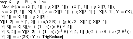
whose first argument X has the following fully general form

$\left\{\left\{\left\{\stackrel{\dot{}}{x}\mathrm{,}\stackrel{\dot{}}{y}\right\}\mathrm{,\; <mtext>\; \hspace{0.17em}\; </mtext>}\left\{\stackrel{⃛}{x}\mathrm{,}\stackrel{⃛}{y}\right\}\right\}\mathrm{,\; <mtext>\; \hspace{0.17em}\; </mtext>}\ddot{z}\mathrm{,\; <mtext>\; \hspace{0.17em}\; </mtext>}\left\{\left\{\stackrel{\dot{}}{u}\mathrm{,}\stackrel{\dot{}}{v}\right\}\mathrm{,\; <mtext>\; \hspace{0.17em}\; </mtext>}\left\{\stackrel{⃛}{u}\mathrm{,}\stackrel{⃛}{v}\right\}\right\}\right\}$ (21)

(the rest of them are self-explanatory). Triple dot indicates cubic terms of the corresponding components. The output computes the location and direction of the ray upon entering the next surface. It can then be used as the first argument of the subsequent call to “step” (with new values of g, R and n), and so one, thus following the ray from one surface to the next, till reaching the end of the optical system. We present some examples of this in due course, but let us first explore what to expect of the final output, after k such steps have been taken.

4. Optical Systems

It is obvious that, starting with $\left\{\left\{\left\{x_0\mathrm{,}{y}_0\right\}\mathrm{,}\left\{\mathrm{0,0}\right\}\right\}\mathrm{,0,}\left\{\left\{u_0\mathrm{,}{v}_0\right\}\mathrm{,}\left\{\mathrm{0,0}\right\}\right\}\right\}$ and advancing through k steps of this procedure, the resulting first two components (of both location and direction) will consist of only linear and cubic terms in $x_0\mathrm{,\; <mtext>\; \hspace{0.17em}\; </mtext>}{y}_0\mathrm{,\; <mtext>\; \hspace{0.17em}\; </mtext>}{u}_0$ and $v_0$. These results must be invariant under each of the following two (with respect to the y-z, and to the x-z plane) reflections, i.e. after simultaneous $x\to -x$, $u\to -u$ (and/or $y\to -y$, $v\to -v$ ) replacement; this reduces the number of potential linear terms from four to two, and cubic terms from twenty to ten, thus:

$\begin{array}{c}{x}_k=A_k{x}_0+C_k{u}_0+E_1^{\left(k\right)}{u}_0^3+E_2^{\left(k\right)}{u}_0{v}_0^2+E_3^{\left(k\right)}{x}_0{u}_0^2+E_4^{\left(k\right)}{x}_0{v}_0^2\\ +E_5^{\left(k\right)}{x}_0^2{u}_0+E_6^{\left(k\right)}{x}_0^3+E_7^{\left(k\right)}{x}_0{y}_0^2+E_8^{\left(k\right)}{y}_0{u}_0{v}_0+E_9^{\left(k\right)}{x}_0{y}_0{v}_0+E_0^{\left(k\right)}{y}_0^2{u}_0\end{array}$ (22)

$\begin{array}{c}{u}_k=B_k{x}_0+D_k{u}_0+F_1^{\left(k\right)}{u}_0^3+F_2^{\left(k\right)}{u}_0{v}_0^2+F_3^{\left(k\right)}{x}_0{u}_0^2+F_4^{\left(k\right)}{x}_0{v}_0^2\\ +F_5^{\left(k\right)}{x}_0^2{u}_0+F_6^{\left(k\right)}{x}_0^3+F_7^{\left(k\right)}{x}_0{y}_0^2+F_8^{\left(k\right)}{y}_0{u}_0{v}_0+F_9^{\left(k\right)}{x}_0{y}_0{v}_0+F_0^{\left(k\right)}{y}_0^2{u}_0\end{array}$ (23)

and their $x\leftrightarrow y$, $u\leftrightarrow v$ analogs. The cubic coefficients are further constrained by rotational symmetry, meaning that all equations must be invariant under the following replacement: $x_0\to x_0\cos \left(\beta \right)-y_0\sin \left(\beta \right)$, $y_0\to x_0\sin \left(\beta \right)+y_0\cos \left(\beta \right)$, $u_0\to u_0\cos \left(\beta \right)-v_0\sin \left(\beta \right)$ and $v_0\to u_0\sin \left(\beta \right)+v_0\cos \left(\beta \right)$. This implies that

$E_1^{\left(k\right)}=E_2^{\left(k\right)}$ (24)

$E_6^{\left(k\right)}=E_7^{\left(k\right)}$ (25)

$E_8^{\left(k\right)}=E_3^{\left(k\right)}-E_4^{\left(k\right)}$ (26)

$E_9^{\left(k\right)}=E_5^{\left(k\right)}-E_0^{\left(k\right)}$ (27)

and their $F^{\left(k\right)}$ analogs. The easiest way to verify these is to use induction: the constraints certainly hold for the initial components (having no cubic terms at all); feeding an X which has a general form of the RHS of (22) and (23), restricted by (24) to (27), into “step”, and checking that the coefficients of the output meet the same restrictions completes the proof (which we leave as an exercise).

Note that the recursive formula for the linear coefficients of the (22/23) transformation can be expressed in a simple matrix form, thus

$\left[\begin{array}{cc}{A}_k& C_k\\ B_k& D_k\end{array}\right]=\left[\begin{array}{cc}1& g_k\\ \frac{1-n_k}{n_k{R}_k}& \frac{R_k+g_k\left(1-n_k\right)}{n_k{R}_k}\end{array}\right]\left[\begin{array}{cc}{A}_{k-1}& C_{k-1}\\ B_{k-1}& D_{k-1}\end{array}\right]$ (28)

which follows from generalization of (6) and (20). Since the determinant of the first RHS matrix is $1/n_k$, and the second RHS matrix is the unit matrix when $k=1$, we get the following expression for the determinant of the left-hand-side matrix

$A_k{D}_k-B_k{C}_k=\frac{1}{{\displaystyle {\prod }_{j=1}^k}{n}_j}$ (29)

These formulas are interesting in their own right, but also essential for the proof of our next statement.

The coefficients of (22/23) are further restricted by the following identities

$E_3^{\left(k\right)}-3E_4^{\left(k\right)}=\left({\displaystyle {\sum }_{i=1}^k}\frac{1}{R_i{\displaystyle {\prod }_{j=1}^{i-1}}{n}_j}-{\displaystyle {\sum }_{i=1}^{k-1}}\frac{1}{R_i{\displaystyle {\prod }_{j=1}^i}{n}_j}\right)\cdot C_k$ (30)

$E_5^{\left(k\right)}-3E_0^{\left(k\right)}=-\left({\displaystyle {\sum }_{i=1}^k}\frac{1}{R_i{\displaystyle {\prod }_{j=1}^{i-1}}{n}_j}-{\displaystyle {\sum }_{i=1}^{k-1}}\frac{1}{R_i{\displaystyle {\prod }_{j=1}^i}{n}_j}\right)\cdot A_k$ (31)

$F_3^{\left(k\right)}-3F_4^{\left(k\right)}=\left({\displaystyle {\sum }_{i=1}^k}\frac{1}{R_i{\displaystyle {\prod }_{j=1}^{i-1}}{n}_j}-{\displaystyle {\sum }_{i=1}^k}\frac{1}{R_i{\displaystyle {\prod }_{j=1}^i}{n}_j}\right)\cdot D_k$ (32)

$F_5^{\left(k\right)}-3F_0^{\left(k\right)}=-\left({\displaystyle {\sum }_{i=1}^k}\frac{1}{R_i{\displaystyle {\prod }_{j=1}^{i-1}}{n}_j}-{\displaystyle {\sum }_{i=1}^k}\frac{1}{R_i{\displaystyle {\prod }_{j=1}^i}{n}_j}\right)\cdot B_k$ (33)

Proof. To prove (30) and (32), we first re-state them in the following form

$\mathcal{H}⊳x_k=\left(S_k+\frac{1}{R_k{\displaystyle {\prod }_{j=1}^k}{n}_j}\right)C_k$ (34)

$\mathcal{H}⊳u_k=S_k{D}_k$ (35)

where $\mathcal{H}⊳$, applied to a cubic polynomial in $x_0\mathrm{,}{y}_0\mathrm{,}{u}_0$ and $v_0$, returns the coefficient of $x_0{u}_0^2$ minus three times the coefficient of $x_0{v}_0^2$, and $S_k$ is the expression in parentheses on the RHS of (32).

Secondly, since

${\stackrel{\dot{}}{x}}_k=A_k{x}_0+C_k{u}_0$ (36)

${\stackrel{\dot{}}{u}}_k=B_k{x}_0+D_k{u}_0$ (37)

(and their $x\leftrightarrow y$, $u\leftrightarrow v$ analogs), it is easy to verify that

$\mathcal{H}⊳\left({\stackrel{\dot{}}{x}}_k^2+{\stackrel{\dot{}}{y}}_k^2\right){\stackrel{\dot{}}{x}}_k=0$ (38)

$\mathcal{H}⊳\left({\stackrel{\dot{}}{x}}_k{\stackrel{\dot{}}{u}}_k+{\stackrel{\dot{}}{y}}_k{\stackrel{\dot{}}{v}}_k\right){\stackrel{\dot{}}{x}}_k=-C_k\left(A_k{D}_k-B_k{C}_k\right)=-\frac{C_k}{{\displaystyle {\prod }_{j=1}^k}{n}_j}$ (39)

$\mathcal{H}⊳\left({\stackrel{\dot{}}{u}}_k^2+{\stackrel{\dot{}}{v}}_k^2\right){\stackrel{\dot{}}{x}}_k=-2D_k\left(A_k{D}_k-B_k{C}_k\right)=-\frac{2D_k}{{\displaystyle {\prod }_{j=1}^k}{n}_j}$ (40)

$\mathcal{H}⊳\left({\stackrel{\dot{}}{x}}_k^2+{\stackrel{\dot{}}{y}}_k^2\right){\stackrel{\dot{}}{u}}_k=2C_k\left(A_k{D}_k-B_k{C}_k\right)=\frac{2C_k}{{\displaystyle {\prod }_{j=1}^k}{n}_j}$ (41)

$\mathcal{H}⊳\left({\stackrel{\dot{}}{x}}_k{\stackrel{\dot{}}{u}}_k+{\stackrel{\dot{}}{y}}_k{\stackrel{\dot{}}{v}}_k\right){\stackrel{\dot{}}{u}}_k=D_k\left(A_k{D}_k-B_k{C}_k\right)=\frac{D_k}{{\displaystyle {\prod }_{j=1}^k}{n}_j}$ (42)

$\mathcal{H}⊳\left({\stackrel{\dot{}}{u}}_k^2+{\stackrel{\dot{}}{v}}_k^2\right){\stackrel{\dot{}}{u}}_k=0$ (43)

We now proceed by induction: (34) and (35) are certainly true for $k=0$ (the initial values of location and direction have no cubic terms), and the statements are assumed correct for k. The objective is to prove that they must then hold for $k+1$.

We get, for the first component of the generalized (i.e. $0\to k$ and $1\to k+1$ ) version of (6),

$\mathcal{H}⊳x_{k+1}=\mathcal{H}⊳\left[x_k+g_{k+1}{u}_k+\left(\frac{{\stackrel{\dot{}}{x}}_k^2+{\stackrel{\dot{}}{y}}_k^2+2g_{k+1}\left({\stackrel{\dot{}}{x}}_k{\stackrel{\dot{}}{u}}_k+{\stackrel{\dot{}}{y}}_k{\stackrel{\dot{}}{v}}_k\right)}{2R_{k+1}}-\frac{{\stackrel{\dot{}}{x}}_k^2+{\stackrel{\dot{}}{y}}_k^2}{2R_k}\right){\stackrel{\dot{}}{u}}_k\right]$ (44)

based on the fact that the $g_{k+1}^2$ proportionate and b proportionate terms contribute zero. The RHS is equal to

$\begin{array}{l}\left(S_k+\frac{1}{R_k{\displaystyle {\prod }_{j=1}^k}{n}_j}\right)C_k+g_{k+1}{S}_k{D}_k+\frac{C_k+g_{k+1}{D}_k}{R_{k+1}{\displaystyle {\prod }_{j=1}^k}{n}_j}-\frac{C_k}{R_k{\displaystyle {\prod }_{j=1}^k}{n}_j}\\ =\left(S_k+\frac{1}{R_{k+1}{\displaystyle {\prod }_{j=1}^k}{n}_j}\right)C_{k+1}=\left(S_{k+1}+\frac{1}{R_{k+1}{\displaystyle {\prod }_{j=1}^{k+1}}{n}_j}\right)C_{k+1}\end{array}$ (45)

which proves (30).

Similarly, based on the generalized version of (20),

$\begin{array}{l}\mathcal{H}⊳u_{k+1}\\ =\mathcal{H}⊳[\frac{u_k}{n_{k+1}}+\frac{\left(1-n_{k+1}\right)x_{k+1}}{n_{k+1}{R}_{k+1}}\\ +\frac{1-n_{k+1}}{n_{k+1}^2{R}_{k+1}}\left(\frac{{\stackrel{\dot{}}{x}}_k{\stackrel{\dot{}}{u}}_k+{\stackrel{\dot{}}{y}}_k{\stackrel{\dot{}}{v}}_k+g_{k+1}\left({\stackrel{\dot{}}{u}}_k^2+{\stackrel{\dot{}}{v}}_k^2\right)}{R_{k+1}}+\frac{{\stackrel{\dot{}}{u}}_k^2+{\stackrel{\dot{}}{v}}_k^2}{2}\right){\stackrel{\dot{}}{x}}_{k+1}]\end{array}$

$\begin{array}{l}=\left(S_{k+1}+\frac{1}{R_{k+1}{\displaystyle {\prod }_{j=1}^{k+1}}{n}_j}-\frac{1}{R_{k+1}{\displaystyle {\prod }_{j=1}^k}{n}_j}\right)\frac{D_k}{n_{k+1}}\\ +\frac{1-n_{k+1}}{n_{k+1}{R}_{k+1}}\left(S_{k+1}+\frac{1}{R_{k+1}{\displaystyle {\prod }_{j=1}^{k+1}}{n}_j}\right)\left(C_k+g_{k+1}{D}_k\right)\\ +\frac{1-n_{k+1}}{n_{k+1}^2{R}_{k+1}}\left(-\frac{C_k}{R_{k+1}{\displaystyle {\prod }_{j=1}^k}{n}_j}-\frac{\left(2g_{k+1}+R_{k+1}\right)D_k}{R_{k+1}{\displaystyle {\prod }_{j=1}^k}{n}_j}+\frac{g_{k+1}{D}_k}{R_{k+1}{\displaystyle {\prod }_{j=1}^k}{n}_j}\right)\\ =S_{k+1}\left(\frac{1-n_{k+1}}{n_{k+1}{R}_{k+1}}{C}_k+\frac{R_{k+1}+g_{k+1}\left(1-n_{k+1}\right)}{n_{k+1}{R}_{k+1}}{D}_k\right)=S_{k+1}{D}_{k+1}\end{array}$ (46)

thus proving (32). Note that we have replaced $S_k$ by the correspondingly adjusted $S_{k+1}$ (the first big parentheses); also that this time it is the a proportionate term which contributes zero.

Proving (31) and (33) is then done in a practically identical way; one has only to modify the definition $\mathcal{H}⊳$ (to: the coefficient of $x_0^2{u}_0$ minus three times the coefficient of $y_0^2{u}_0$ ), and replace C by A and D by B.n

5. Image Construction

Without a loss of generality, we now assume that the object is placed at $\langle x\mathrm{,0,0}\rangle$, and trace a ray with an initial direction of

$\langle v\cos \left(\beta \right)\mathrm{,}v\sin \left(\beta \right)\mathrm{,1}-v^2/2\rangle$ (47)

This will make all terms containing a power of $y_0$ equal to zero in the (22/23) equations, thus simplifying them to read

$\begin{array}{l}{x}_k=A_{k}x+C_{k}v\cos \left(\beta \right)+E_1^{\left(k\right)}{v}^3\cos \left(\beta \right)+E_3^{\left(k\right)}x{v}^2\frac{1+\cos \left(2\beta \right)}{2}\\ +E_4^{\left(k\right)}x{v}^2\sin {\left(\beta \right)}^2+E_5^{\left(k\right)}{x}^{2}v\cos \left(\beta \right)+E_6^{\left(k\right)}{x}^3\\ y_k=C_{k}v\sin \left(\beta \right)+E_1^{\left(k\right)}{v}^3\sin \left(\beta \right)+E_8^{\left(k\right)}x{v}^2\frac{\sin \left(2\beta \right)}{2}+E_0^{\left(k\right)}{x}^{2}v\sin \left(\beta \right)\end{array}$ (48)

and analogous expansions of $u_k$ and $v_k$.

Once we have reached the last (say k^th) surface of the optical system, we create an imaginary, flat ( $R_{k+1}=\infty$ ), $k+1^{\text{st}}$ surface at a distance $g_{k+1}$ from the last surface’s apex (the corresponding $n_{k+1}$ at the k^th surface is equal to 1, since the optical medium remains the same); we choose $g_{k+1}$ in such a way to make $C_{k+1}$ equal to zero, resulting in all rays emanating from our image converge (to linear accuracy) to a single point. Since, based on (28) with $k\to k+1$,

$C_{k+1}=C_k+g_{k+1}{D}_k$ (49)

this is achieved by taking $g_{k+1}=-\frac{C_k}{D_k}$. Thus, any object with the initial z coordinate equal to 0 (thus defining the object plane—objects located in this plane form what we call a scenery) will come into a sharp (i.e. to the first order approximation) focus in thus created image plane.

Nevertheless, the cubic terms of the final location of our image indicate that the convergence is not perfect: the image is either slightly misplaced from its ideal location (thus distorting the shape of the original scenery), or smeared in a variety of ways. Since we have made $C_{k+1}$ equal to zero, this implies that $E_3^{\left(k+1\right)}=3E_4^{\left(k+1\right)}$, which, together with (26), enables us to further simplify coordinates of the final image’s location to

$\begin{array}{l}{x}_{k+1}=A_{k+1}x+E_1^{\left(k+1\right)}{v}^3\cos \left(\beta \right)+E_4^{\left(k+1\right)}x{v}^2\left(2+\cos \left(2\beta \right)\right)\\ +E_5^{\left(k+1\right)}{x}^{2}v\cos \left(\beta \right)+E_6^{\left(k+1\right)}{x}^3\\ y_{k+1}=E_1^{\left(k+1\right)}{v}^3\sin \left(\beta \right)+E_4^{\left(k+1\right)}x{v}^2\sin \left(2\beta \right)+E_0^{\left(k+1\right)}{x}^{2}v\sin \left(\beta \right)\end{array}$ (50)

6. Aberrations

Let us now explore how these cubic terms affect the quality of the image.

· The $x^3$ term displaces the location of the image away from (towards)—depending on the sign of $E_6^{\left(k+1\right)}$ —the optical axis; this effect increases with the magnitude of $E_6^{\left(k+1\right)}$, but also with the distance of the image from the axis, thus causing a distortion of the original scenery (see Figure 1).

· The $v^3$ terms smear each image (ideally, a single point) into a small disk whose size is proportional to $E_1^{\left(k+1\right)}$, with most rays concentrated at its center, and of diminishing (with $r^{-3}$, where r is the distance from this center) light intensity towards its edges; this is called spherical aberration and it is the same for all images, regardless of their distance from the optical axis (see Figure 2).

· The $x{v}^2$ terms similarly smear the image into a 60˚ wedge pointing towards the optical axis, with a high-intensity apex at the image’s original location, and of decreasing intensity as it spreads up (see Figure 2); this is the so-called coma—the size of the wedge is proportional not only to $E_4^{\left(k+1\right)}$ but also to its distance from the optical axis.

· The $x^{2}v$ terms have two different manifestations: their average effect, namely

$\frac{E_5^{\left(k+1\right)}+E_0^{\left(k+1\right)}}{2}\cdot x^2\langle v\cos \left(\beta \right)\mathrm{,}v\sin \left(\beta \right)\rangle$ (51)

can be removed by changing the $z=-\frac{C_k}{D_k}$ image plane to

Figure 1. Positive and negative distortion.

Figure 2. Spherical aberration, coma and astigmatism.

$z=-\frac{C_k}{D_k}-\frac{E_5^{\left(k+1\right)}+E_0^{\left(k+1\right)}}{2D_k}\cdot x^2$ (52)

i.e. a slightly curved (spherical, to a sufficient approximation) surface of radius $\frac{D_k}{E_5^{\left(k+1\right)}+E_0^{\left(k+1\right)}}$ (we call it the screen from now on); this aberration is called the medial field curvature.

· The remaining

$\frac{E_5^{\left(k+1\right)}-E_0^{\left(k+1\right)}}{2}\cdot x^2\langle v\cos \left(\beta \right)\mathrm{,}-v\sin \left(\beta \right)\rangle$ (53)

then yields a disk of uniform intensity (on the new screen—it would form an ellipse in the original image plane). The size of the disk is determined by the system’s aperture—see [6], but it is also proportional to the first two factors in (53), thus becoming point-like again for images close to the optical axis.

More interestingly, by further modifying the screen’s curvature (making its radius equal to $\frac{D_k}{2E_5^{\left(k+1\right)}}$ ), we may fully remove the first component of (53), thus making all rays staying in the x-z plane intersect at a single point (their tangential focus), while the remaining rays smear into a straight-line segment in a perpendicular-to-x-z (also known as sagittal) direction. Similarly, when the radius changes to $\frac{D_k}{2E_0^{\left(k+1\right)}}$, it is the perpendicular rays which converge to the sagittal focus, while the rest of them create a line segment in the x direction. This effect is called astigmatism (see Figure 2).

We should now mention that these formulas have been derived assuming a conical pencil of rays whose central ray is parallel to the z axis. But this would often result in most of these rays missing the first spherical surface (which is always of only a finite radial extent). It is therefore important to redirect the cone towards the central part of this surface; this can be achieved by changing (47) to

$\langle v\cos \left(\beta \right)-\frac{x}{g}\mathrm{,}v\sin \left(\beta \right)\mathrm{,}\cdots \rangle$ (54)

so that (to a good approximation) the central ray (properly called chief of primary ray, see [7] ) enters the first surface at its apex. This maximizes the size of the light pencil which will pass through the optical system and build the corresponding image (the situation is actually more complicated—the cone should be directed at the so-called entrance pupil, but discussing this would take us beyond the scope of this article). This will correspondingly change the $E^{\left(k+1\right)}$ coefficients in (50), but it will not change the general form of it; this is easy to prove, and it is also automatically achieved by our Mathematica program.

7. Examples

7.1. Simple Lens

When an optical system consists of more than one lens, finding general formulas for individual aberrations is not feasible (they would be extremely lengthy functions of many parameters). We thus choose to do this only for the simplest possible optical system, namely a single lens with identically shaped surfaces (of radius R and -R) at zero distance from each other (the thin-lens approximation, which works reasonably well when their distance is small). To get the answer, all we need to do is to type:

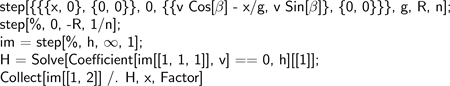
Note that to find $g_{k+1}$ (denoted h and H in the program) of the image plane, we had to eliminate the v term in the linear part of the first component of the image’s location.

Running this code yields the following results: there is zero distortion, while the remaining aberration terms are

$-Q\cdot \langle \left(n+3\right)\cos \left(\beta \right)\mathrm{,}\left(n+1\right)\sin \left(\beta \right)\rangle \mathrm{<mtext>\; \hspace{0.17em}\; </mtext>}{x}^{2}v\text{fieldcurvature/astigmatism}$

$-Q\left(2n+1\right)\left(\frac{g^2}{R}\left(n-1\right)-g\right)\cdot \langle 2+\cos \left(2\beta \right)\mathrm{,}\sin \left(2\beta \right)\rangle \mathrm{<mtext>\; \hspace{0.17em}\; </mtext>}x\mathrm{<mtext>\; \hspace{0.17em}\; </mtext>}{v}^2\text{coma}$ (55)

$-Q\frac{g^2}{R^2}W\cdot \langle \cos \left(\beta \right)\mathrm{,}\sin \left(\beta \right)\rangle \mathrm{<mtext>\; \hspace{0.17em}\; </mtext>}{v}^3\text{sphericalaberration}$

where

$\begin{array}{l}Q=\frac{n-1}{n\left(2g\left(n-1\right)-R\right)}\\ W=g^2\left(2-n-4n^2+4n^3\right)-\left(3n+2\right)\left(2g\left(n-1\right)-R\right)R\end{array}$ (56)

n is the lens’ index of refraction and g is the distance from the object to the first surface.

Note that the largest value of x is given by g multiplied by the so-called field of view, while the largest v is given by the radius of the lens’ x-y extent divided by g; this is important to realize when comparing coefficients of different aberrations.

7.2. Objects at Infinity

When the object’s distance from the optical system (our g₁) is orders of magnitude larger than the size of the system itself, it is convenient to employ a different approach: the object’s location can then be specified by the incoming rays’ direction (they arrive practically parallel to each other), and x and y become the first two coordinates of the point at which any such ray enters the $z=0$ plane.

This necessitates reversing the role of x and v when interpreting the resulting aberrations: the term proportional to v³ now represents distortion while the term which goes with x³ yields spherical aberration, etc. We demonstrate how this works, also using a thin lens, but this time allowing its two surfaces to be of different radius, say R₁ and R₂.

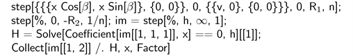
This results in the sum of the following terms

$\frac{R_1{R}_2}{2\left(n-1\right)\left(R_1+R_2\right)}\cdot \langle \mathrm{0,1}\rangle \mathrm{<mtext>\; \hspace{0.17em}\; </mtext>}{v}^3\text{distortion}$

$-\frac{1}{2n}\cdot \langle \left(n+3\right)\cos \left(\beta \right)\mathrm{,}\left(n+1\right)\sin \left(\beta \right)\rangle \mathrm{<mtext>\; \hspace{0.17em}\; </mtext>}x{v}^2\text{fieldcurvature/astigmatism}$ (57)

$\frac{n^2\left(R_1+R_2\right)-\left(n+1\right)R_2}{2n{R}_1{R}_2}\cdot \langle 2+\cos \left(2\beta \right)\mathrm{,}\sin \left(2\beta \right)\rangle \mathrm{<mtext>\; \hspace{0.17em}\; </mtext>}{x}^{2}v\text{coma}$ (58)

$-\frac{n^3{\left(R_1+R_2\right)}^2-n^2{R}_2\left(R_1+R_2\right)-n{R}_1{R}_2+2R_2^2}{2n{R}_1^2{R}_2^2}\cdot \langle \cos \left(\beta \right)\mathrm{,}\sin \left(\beta \right)\rangle \mathrm{<mtext>\; \hspace{0.17em}\; </mtext>}{x}^3$

the last being the spherical aberration.

7.3. Cooke Triplet

This is an old (going back to 1935) design of a camera objective consisting of three lenses (see [6] ); the actual details are obvious from the following Mathematica code (all distances and radii are in mm).

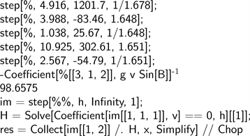
The program yields the usual sum of four aberration terms plus, as a by-product (see [3] ), the focal length of the system (of 98.66 mm).

We have already mentioned that the largest value of x/g is determined by the system’s field of view which is, in this case, about 25 degrees (this can be established by using the same program to follow a principal ray entering the system at 25 degrees and noting that its location upon reaching the last lens is at its very edge—all three lenses have roughly the same diameter of about 200 mm; this implies that a ray entering at a higher angle would not make it through the system). Similarly, the largest value of $v$ is to a good approximation given by the corresponding radius (100 mm), divided by g. To be able to directly compare individual aberrations, we then express them all in powers of

$X=\frac{x}{g\mathrm{<mtext>\; \hspace{0.17em}\; </mtext>}\sin \left(25˚\right)}$ (59)

$V=\frac{v\cdot g}{100}$ (60)

instead of the original x and v. Note that both X and V are now dimensionless, each having the maximum possible value of 1.

This is achieved by extending our program by the following extra line:

The result is still an expression too lengthy to quote here, due to its g dependence. But a simple graph reveals that the expression rather quickly converges (becoming sufficiently accurate when $g>1000\text{mm}$ ) to its $g\to \infty$ limit of

$\begin{array}{l}-\langle \mathrm{0.166,0}\rangle X^3-\langle 0.202\cos \left(\beta \right)\mathrm{,0.278}\sin \left(\beta \right)\rangle X^{2}V\\ -0.050\cdot \langle 2+\cos \left(2\beta \right)\mathrm{,}\sin \left(2\beta \right)\rangle X{V}^2-0.074\cdot \langle \cos \left(\beta \right)\mathrm{,}\sin \left(\beta \right)\rangle V^3\end{array}$

where all coefficients are in mm. This should be compared to the size of the actual image, which our program locates at

$-\langle \mathrm{41.694,0}\rangle X$ (61)

8. Conclusion

We would like to reiterate that this article has focused on a single issue of third-order aberrations of spherically symmetric system of lenses, and has deliberately avoided many other important issues related to optical-system design. We also acknowledge that the ultimate goal of understanding aberrations is to be able to design optical systems which minimize these; something we have not attempted in this article since this goes well beyond its scope. We have also skipped discussing yet another important, so-called chromatic aberration, which is due to the index of refraction changing with the color of the light. We have similarly avoided any mention of wavelike nature of light, and the limitations this imposes on forming an image of an object. Our bibliography lists several books (e.g. [4] and [7] ) which provide more information on many of the topics left out by this article.

Conflicts of Interest

The author declares no conflicts of interest regarding the publication of this paper.

References

[1]	Pedrotti, F.L., Pedrotti, L.M. and Pedrotti, L.S. (2017) Introduction to Optics. 3rd Edition, Cambridge University Press, Cambridge. https://doi.org/10.1017/9781108552493
[2]	Welford, W.T. (1974) Aberrations of the Symmetrical Optical Systems. Academic Press, New York.
[3]	Vrbik, J. (2020) Geometrical Optics from the Ground Up. Applied Mathematics, 11, 1021-1040. https://doi.org/10.4236/am.2020.1110068
[4]	Herzberger, M. (1958) Modern Geometrical Optics. Interscience Publishers, New York.
[5]	Buchdahl, H.A. (1993) An Introduction to Hamiltonian Optics. Dover Publications, New York.
[6]	Smith, W.J. (2008) Modern Optical Engineering. 4th Edition. McGraw-Hill, New York.
[7]	Mahajan, V.N. (1999) Optical Imaging and Aberrations, Part I: Ray Geometrical Optics. SPIE Press, Washington DC.