A Single Server Queue with Coxian-2 Service and One-Phase Vacation (M/C-2/M/1 Queue)

Zeyad R. Al-Rawi¹, Khalid M. S. Al Shboul²

¹Al-Rasheed University College, Baghdad, Iraq.
²Statistical Center, Abu Dhabi, UAE.

DOI: 10.4236/ojapps.2021.116056                

Abstract

In this paper, we study a single server queueing system with Coxian-2 service.  In Particular, we study M/C-2/M/1 queue with Coxian-2 service and exponential vacation. We assume that units (customers) arrive at the system one by one in a Poisson process and the server provides one-by-one service based on first in first out (FIFO) rule. We obtained the steady state queue size distributions in terms of the probability generating functions, the average number of customers and their average waiting time in the system as well as in the queue.

Keywords

Single Server Queues, Poisson Arrivals, Coxian-2 Distribution, Time Depending Solution, Steady State Solution

1. Introduction

In queueing theory we study situations where units of some kind arrive at a service facility for receiving service, some of the units having to wait for service, and go out after service. A queue or a waiting line develops when the service facility cannot deal with the number of units requiring service.

A system is generally defined as something that has an input, output and transformation process, which changes the input into the output. The study of a queuing system provides us with some characteristics that can be used to measure the performance of the system, like the proportion of time the service channel is idle, the proportion of time the service channel is busy and the average waiting time of a customer. Using these and similar measures one can predict what will happen if certain changes are made in the components of the system.

For many queueing systems the queue discipline that is used is first in, first out “FIFO”. Other queue disciplines are last in, first out “LIFO” or there could be a priority service as is common in hospital emergency cases. In this paper we assume FIFO queue discipline.

Coxian-2 Distribution

A random variable X is said to have a Coxian-2 distribution if X can be

represented by $X=\{\begin{array}{l}{X}_1+X_2\text{with probability}b\\ X_1\text{with probability1}-b\end{array}$

where $X_1$ and $X_2$ are independent random variables having exponential

distribution with respective mean $\frac{1}{{\mu }_1}$ and $\frac{1}{{\mu }_2}$.

The probability density function of the Coxian-2 distribution random variable

X is given by $f\left(t\right)=\{\begin{array}{l}{p}_1{\mu }_1{\text{e}}^{-{\mu }_{1}t}+\left(1-p_1\right){\mu }_2{\text{e}}^{-{\mu }_{2}t}\text{if}{\mu }_1\ne {\mu }_2,\\ p_1{\mu }_1{\text{e}}^{-{\mu }_{1}t}+\left(1-p_1\right){\mu }_1^{2}t{\text{e}}^{-{\mu }_{1}t}\text{if}{\mu }_1={\mu }_2\end{array}$

where $p_1=1-b{\mu }_1/\left({\mu }_1-{\mu }_2\right)$ if ${\mu }_1\ne {\mu }_2$ and $p_1=1-b$ if ${\mu }_1={\mu }_2$.

For more details see Tijms [1].

In recent years, vacation queues have been developed as an important area of queueing theory. In classical queueing theory it was assumed that the server is always available in the system. However, this is not true in many real life situations. In many queueing systems such as the large production systems, computer systems or communication networks, there may be a need to stop the system from time to time for routine maintenance or for overhauling. Recently many researchers including Crammer [2], Doshi [3], Keilson and Servi [4], Shanthikumar [5], Madan and Saleh [6] [7] and Madan, Abu-Dayyeh and Tayyan [8] have studied some such queueing systems with server vacations.

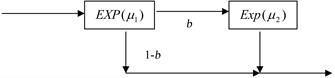
In this paper we study the M/C-2/M/1 queue with Poisson arrivals Coxian-2 service and exponential vacation. Whenever a customer takes a service, his service time is a random variable distributed as Coxian-2. Further, we assume that after every service the server may take a vacation of random length with probability p or may continue the next service with probability (1-p). Whenever the server takes a vacation, his vacation time is distributed exponentially. We have obtained time-dependent as well as steady state queue size distribution. In addition, for the steady state we find the mean queue size, the mean system size and the mean waiting time of a customer.

2. Assumptions, Definitions and Equations Governing the System

In this work we assume that

1) Customers arrive to the system in a Poisson pattern with mean arrival rate $\lambda$.

2) Phase-k service is exponential with mean service time $\frac{1}{{\mu }_k}$, $k=1,2$.

3) The server’s vacation period has an exponential distribution with mean

vacation time $\frac{1}{\beta }$.

4) All random variables involved in the system such as the inter-arrival times of customers, the service times of the customers and the vacation times of the server are independent of each other.

Also we define.

${{\rm P}}_n^k\left(t\right)$ : - Probability that at time t there are n units (customers) in the queue excluding one unit in phase-k service, $k=1,2$ ; $n=0,1,2,\cdots$

$Q\left(t\right)$ : - Probability that at time t there is no unit in the queue and the server is idle.

$V_n\left(t\right)$ : - Probability that at time t there are n units in the queue and the server is on vacation.

p: - Probability that the server takes a vacation after completion of service.

Then we have the following set of equations:

$\begin{array}{l}{{\rm P}}_n^1\left(t+\Delta t\right)={{\rm P}}_n^1\left(t\right)\left(1-\lambda \Delta t\right)\left(1-{\mu }_1\Delta t\right)+{{\rm P}}_{n-1}^1\left(t\right)\left(\lambda \Delta t\right)\left(1-{\mu }_1\Delta t\right)\\ +{{\rm P}}_{n+1}^1\left(t\right)\left(1-\lambda \Delta t\right)\left(1-b\right)\left({\mu }_1\Delta t\right)\left(1-p\right)\\ +{{\rm P}}_{n+1}^2\left(t\right)\left(1-\lambda \Delta t\right)\left({\mu }_2\Delta t\right)\left(1-p\right)\\ +V_{n+1}\left(t\right)\left(1-\lambda \Delta t\right)\beta \Delta t,n\ge 1\end{array}$ (1)

$\begin{array}{c}{{\rm P}}_0^1\left(t+\Delta t\right)={{\rm P}}_0^1\left(t\right)\left(1-\lambda \Delta t\right)\left(1-{\mu }_1\Delta t\right)+{{\rm P}}_1^1\left(t\right)\left(1-\lambda \Delta t\right)\left(1-b\right)\left({\mu }_1\Delta t\right)\left(1-p\right)\\ +{{\rm P}}_1^2\left(t\right)\left(1-\lambda \Delta t\right)\left({\mu }_2\Delta t\right)\left(1-p\right)+V_1\left(t\right)\left(1-\lambda \Delta t\right)\beta \Delta t+Q\left(t\right)\lambda \Delta t,\end{array}$ (2)

$\begin{array}{l}{{\rm P}}_n^2\left(t+\Delta t\right)={{\rm P}}_n^2\left(t\right)\left(1-\lambda \Delta t\right)\left(1-{\mu }_2\Delta t\right)+{{\rm P}}_{n-1}^2\left(t\right)\left(\lambda \Delta t\right)\left(1-{\mu }_2\Delta t\right)\\ +{{\rm P}}_n^1\left(t\right)\left(1-\lambda \Delta t\right)\left({\mu }_1\Delta t\right)b,n\ge 1\end{array}$ (3)

${{\rm P}}_0^2\left(t+\Delta t\right)={{\rm P}}_0^2\left(t\right)\left(1-\lambda \Delta t\right)\left(1-{\mu }_2\Delta t\right)+{{\rm P}}_0^1\left(t\right)\left(1-\lambda \Delta t\right)\left({\mu }_1\Delta t\right)b,$ (4)

$\begin{array}{l}{V}_n\left(t+\Delta t\right)=V_n\left(t\right)\left(1-\lambda \Delta t\right)\left(1-\beta \Delta t\right)+V_{n-1}\left(t\right)\left(\lambda \Delta t\right)\left(1-\beta \Delta t\right)\\ +{{\rm P}}_n^2\left(t\right)\left(1-\lambda \Delta t\right)\left({\mu }_2\Delta t\right)p+{{\rm P}}_n^1\left(t\right)\left(1-\lambda \Delta t\right)\left({\mu }_1\Delta t\right)\left(1-b\right)p,n\ge 1\end{array}$ (5)

$\begin{array}{c}{V}_0\left(t+\Delta t\right)=V_0\left(t\right)\left(1-\lambda \Delta t\right)\left(1-\beta \Delta t\right)+{{\rm P}}_0^2\left(t\right)\left(1-\lambda \Delta t\right)\left({\mu }_2\Delta t\right)p\\ +{{\rm P}}_0^1\left(t\right)\left(1-\lambda \Delta t\right)\left({\mu }_1\Delta t\right)\left(1-b\right)p,\end{array}$ (6)

$\begin{array}{c}Q\left(t+\Delta t\right)=Q\left(t\right)\left(1-\lambda \Delta t\right)+{{\rm P}}_0^1\left(t\right)\left(1-\lambda \Delta t\right)\left({\mu }_1\Delta t\right)\left(1-b\right)\left(1-p\right)\\ +{{\rm P}}_0^2\left(t\right)\left(1-\lambda \Delta t\right)\left({\mu }_2\Delta t\right)\left(1-p\right)+V_0\left(t\right)\left(1-\lambda \Delta t\right)\beta \Delta t,\end{array}$ (7)

In order to give a detailed reasoning needed to get the above equations, we shall explain how Equation (1) has been obtained. We connect the system probabilities at time t with those at timet + Δt by considering ${{\rm P}}_n^1\left(t+\Delta t\right)$ which means the probability that there are n units at time t + Δt excluding one unit in phase-1 of the service. Then we have the following four mutually exclusive cases:

1) At time t, there are n units in the queue excluding one unit in phase-1 service and there is no arrival and no service completion during $\left(t,t+\Delta t\right]$. This case has the joint probability ${{\rm P}}_n^1(t)\left(1-\lambda \Delta t\right)\left(1-{\mu }_1\Delta t\right)$.

2) At time t, there are n − 1 units in the queue excluding one unit in phase-1 service and there is one arrival and no service completion during $\left(t,t+\Delta t\right]$. This case has the joint probability ${{\rm P}}_{n-1}^1\left(t\right)\left(\lambda \Delta t\right)\left(1-{\mu }_1\Delta t\right)$.

3) At time t, there are n + 1 units in the queue excluding one unit in phase-1 service and there is no arrival, one service completion during $\left(t,t+\Delta t\right]$ and the customer decides not to take phase-2 of service, also the server doesn’t take vacation with probability (1-p). This case has the joint probability ${{\rm P}}_{n+1}^1\left(t\right)\left(1-\lambda \Delta t\right)\left(1-b\right)\left({\mu }_1\Delta t\right)\left(1-p\right)$.

4) At time t, there are n + 1 units in the queue excluding one unit in phase-2 service and there is no arrival, one service completion during $\left(t,t+\Delta t\right]$, and the server does not take vacation with probability (1-p). This case has the joint probability ${{\rm P}}_{n+1}^2\left(t\right)\left(1-\lambda \Delta t\right)\left({\mu }_2\Delta t\right)\left(1-p\right)$.

5) At time t, there are n + 1 units in the queue and the server is on vacation, and no arrival, one vacation complete during $\left(t,t+\Delta t\right]$. This case has the joint probability $V_{n+1}\left(t\right)\left(1-\lambda \Delta t\right)\beta \Delta t$.

After rearranging the terms in the above equations and letting $\Delta t\to 0$ we obtain the following set of differential equations:

$\begin{array}{l}\frac{\text{d}}{\text{d}t}{{\rm P}}_n^1\left(t\right)=-\left(\lambda +{\mu }_1\right){{\rm P}}_n^1\left(t\right)+\lambda {{\rm P}}_{n-1}^1\left(t\right)+\left(1-b\right)\left(1-p\right){\mu }_1{{\rm P}}_{n+1}^1\left(t\right)\\ +\left(1-p\right){\mu }_2{{\rm P}}_{n+1}^2\left(t\right)+\beta V_{n+1}\left(t\right),n\ge 1\end{array}$ (8-1)

$\begin{array}{c}\frac{\text{d}}{\text{d}t}{{\rm P}}_0^1\left(t\right)=-\left(\lambda +{\mu }_1\right){{\rm P}}_0^1\left(t\right)+\left(1-b\right)\left(1-p\right){\mu }_1{{\rm P}}_1^1\left(t\right)\\ +\left(1-p\right){\mu }_2{{\rm P}}_1^2\left(t\right)+\beta V_1\left(t\right)+\lambda Q\left(t\right),\end{array}$ (8-2)

$\frac{\text{d}}{\text{d}t}{{\rm P}}_n^2\left(t\right)=-\left(\lambda +{\mu }_2\right){{\rm P}}_n^2\left(t\right)+\lambda {{\rm P}}_{n-1}^2\left(t\right)+b{\mu }_1{{\rm P}}_n^1\left(t\right),n\ge 1$ (8-3)

$\frac{\text{d}}{\text{d}t}{{\rm P}}_0^2\left(t\right)=-\left(\lambda +{\mu }_2\right){{\rm P}}_0^2\left(t\right)+b{\mu }_1{{\rm P}}_0^1\left(t\right),$ (8-4)

$\frac{\text{d}}{\text{d}t}{V}_n\left(t\right)=-\left(\lambda +\beta \right)V_n\left(t\right)+\lambda V_{n-1}\left(t\right)+p{\mu }_2{{\rm P}}_n^2\left(t\right)+\left(1-b\right)p{\mu }_1{{\rm P}}_n^1\left(t\right),n\ge 1$ (8-5)

$\frac{\text{d}}{\text{d}t}{V}_0\left(t\right)=-\left(\lambda +\beta \right)V_0\left(t\right)+p{\mu }_2{{\rm P}}_0^2\left(t\right)+\left(1-b\right)p{\mu }_1{{\rm P}}_0^1\left(t\right),$ (8-6)

$\frac{\text{d}}{\text{d}t}Q\left(t\right)=-\lambda Q\left(t\right)+\left(1-b\right)\left(1-p\right){\mu }_1{{\rm P}}_0^1\left(t\right)+\left(1-p\right){\mu }_2{{\rm P}}_0^2\left(t\right)+\beta V_0\left(t\right).$ (8-7)

3. Time Dependent Solution

Assuming that initially there are no customers in the system and the server is idle, we have the following initial conditions:

${{\rm P}}_n^k\left(0\right)=0,k=1,2$, $V_n\left(0\right)=0,\forall n\ge 0$, $Q\left(0\right)=1$ (9)

Now by taking Laplace transformation of Equations [(8-1)-(8-7)] and using (9) we get the following:

$\begin{array}{c}s{{\rm P}}_n^{*1}\left(s\right)-{{\rm P}}_n^1\left(0\right)=-\left(\lambda +{\mu }_1\right){{\rm P}}_n^{*1}\left(s\right)+\lambda {{\rm P}}_{n-1}^{*1}\left(s\right)+\left(1-b\right)\left(1-p\right){\mu }_1{{\rm P}}_{n+1}^{*1}\left(s\right)\\ +\left(1-p\right){\mu }_2{{\rm P}}_{n+1}^{*2}\left(s\right)+\beta V_{n+1}^{*}(\; s\; )\end{array}$

$\begin{array}{l}\Rightarrow \left(s+\lambda +{\mu }_1\right){{\rm P}}_n^{*1}\left(s\right)=\lambda {{\rm P}}_{n-1}^{*1}\left(s\right)+\left(1-b\right)\left(1-p\right){\mu }_1{{\rm P}}_{n+1}^{*1}\left(s\right)\\ +\left(1-p\right){\mu }_2{{\rm P}}_{n+1}^{*2}\left(s\right)+\beta V_{n+1}^{*}\left(s\right),n\ge 1\end{array}$ (10-1)

$\begin{array}{l}\left(s+\lambda +{\mu }_1\right){{\rm P}}_0^{*1}\left(s\right)\\ =\left(1-b\right)\left(1-p\right){\mu }_1{{\rm P}}_1^{*1}\left(s\right)+\left(1-p\right){\mu }_2{{\rm P}}_1^{*2}\left(s\right)+\beta V_1^{*}\left(s\right)+\lambda Q^{*}\left(s\right)\end{array}$ (10-2)

$\left(s+\lambda +{\mu }_2\right){{\rm P}}_n^{*2}\left(s\right)=\lambda {{\rm P}}_{n-1}^{*2}\left(s\right)+b{\mu }_1{{\rm P}}_n^{*1}\left(s\right),n\ge 1$ (10-3)

$\left(s+\lambda +{\mu }_2\right){{\rm P}}_0^{*2}\left(s\right)=b{\mu }_1{{\rm P}}_0^{*1}\left(s\right)$ (10-4)

$\left(s+\lambda +\beta \right)V_n^{*}\left(s\right)=\lambda V_{n-1}^{*}\left(s\right)+p{\mu }_2{{\rm P}}_n^{*2}\left(s\right)+p\left(1-b\right){\mu }_1{{\rm P}}_n^{*1}\left(s\right),n\ge 1$ (10-5)

$\left(s+\lambda +\beta \right)V_0^{*}\left(s\right)=p{\mu }_2{{\rm P}}_0^{*2}\left(s\right)+p\left(1-b\right){\mu }_1{{\rm P}}_0^{*1}\left(s\right)$ (10-6)

$\left(s+\lambda \right)Q^{*}\left(s\right)=\left(1-b\right)\left(1-p\right){\mu }_1{{\rm P}}_0^{*1}\left(s\right)+\left(1-p\right){\mu }_2{{\rm P}}_0^{*2}\left(s\right)+\beta V_0^{*}\left(s\right)+1$ (10-7)

Next, we define the following probability generating functions in terms of their Laplace transforms:

${{\rm P}}^{*k}\left(z,s\right)={\displaystyle \underset{n=0}{\overset{\infty }{\sum }}{{\rm P}}_n^{*k}\left(s\right)z^n},k=1,2$ (11)

$V^{*}\left(z,s\right)={\displaystyle \underset{n=0}{\overset{\infty }{\sum }}{V}_n^{*}\left(s\right)z^n}$ (12)

where z is a dummy variable and $\left|z\right|\le 1$.

Multiply Equation (10-1) by $z^{n+1}$ and sum over n = 1 to ¥, and multiply (10-2) by z, then add them together we get

$\begin{array}{l}\left(s+\lambda +{\mu }_1\right){\displaystyle \underset{n=0}{\overset{\infty }{\sum }}{{\rm P}}_n^{*1}\left(s\right)z^{n+1}}\\ =\lambda z^2{\displaystyle \underset{n=0}{\overset{\infty }{\sum }}{{\rm P}}_n^{*1}\left(s\right)z^n+}\left(1-b\right)\left(1-p\right){\mu }_1{\displaystyle \underset{n=1}{\overset{\infty }{\sum }}{{\rm P}}_n^{*1}\left(s\right)z^n}\\ +\left(1-p\right){\mu }_2{\displaystyle \underset{n=1}{\overset{\infty }{\sum }}{{\rm P}}_n^{*2}\left(s\right)z^n}+\beta {\displaystyle \underset{n=1}{\overset{\infty }{\sum }}{V}_n^{*}\left(s\right)z^n}+Q^{*}\left(s\right)z\end{array}$

And by using the terms defined by (11) and (12), we obtain

$\begin{array}{l}z{{\rm P}}^{*1}\left(z,s\right)\left(s+\lambda +{\mu }_1-\lambda z\right)\\ =\left(1-b\right)\left(1-p\right){\mu }_1{{\rm P}}^{*1}\left(z,s\right)+\left(1-p\right){\mu }_2{{\rm P}}^{*2}\left(z,s\right)+\beta V^{*}\left(z,s\right)+\lambda z{Q}^{*}\left(s\right)\\ -\left[\left(1-b\right)\left(1-p\right){\mu }_1{{\rm P}}_0^{*1}\left(s\right)+\left(1-p\right){\mu }_2{{\rm P}}_0^{*2}\left(s\right)+\beta V_0^{*}\left(s\right)\right]\end{array}$ (13)

Now using Equations (10-7), (13) can be re-written as

$\begin{array}{l}{{\rm P}}^{*1}\left(z,s\right)\left[z\left(s+\lambda +{\mu }_1-\lambda z\right)-\left(1-b\right)\left(1-p\right){\mu }_1\right]\\ =\left(1-p\right){\mu }_2{{\rm P}}^{*2}\left(z,s\right)+\beta V^{*}\left(z,s\right)+Q^{*}\left(s\right)\left(\lambda z-s-\lambda \right)+1\end{array}$ (14)

Next multiply (10-3) by zⁿ and sum over n = 1 to ¥, and (10-4) to the result. Thus we have

${{\rm P}}^{*2}\left(z,s\right)\left(s+\lambda +{\mu }_2-\lambda z\right)=b{\mu }_1{{\rm P}}^{*1}\left(z,s\right)$ (15)

Then multiplying Equation (10-5) by zⁿ and summing over n = 1 to ¥, then adding the result to (10-6) will give:

$V^{*}\left(z,s\right)\left(s+\lambda +\beta -\lambda z\right)=p{\mu }_2{{\rm P}}^{*2}\left(z,s\right)+p\left(1-b\right){\mu }_1{{\rm P}}^{*1}\left(z,s\right)$ (16)

Now, on solving Equations (14)-(16) using Cramer’s rule we get:

${{\rm P}}^{*1}\left(z,s\right)=\frac{\left[Q^{*}\left(s\right)\left(\lambda z-\lambda -s\right)+1\right]\left(s+{\mu }_2+\lambda -\lambda z\right)\left(s+\beta +\lambda -\lambda z\right)}{D\left(s,z\right)}$ (17)

${{\rm P}}^{*2}\left(z,s\right)=\frac{b{\mu }_1\left[Q^{*}\left(s\right)\left(\lambda z-\lambda -s\right)+1\right]\left(s+\beta +\lambda -\lambda z\right)}{D\left(s,z\right)}$ (18)

$V^{*}\left(z,s\right)=\frac{\left[Q^{*}\left(s\right)\left(\lambda z-\lambda -s\right)+1\right]\left[bp{\mu }_1{\mu }_2+p\left(1-b\right){\mu }_1\left(s+{\mu }_2+\lambda -\lambda z\right)\right]}{D\left(s,z\right)}$ (19)

where

$\begin{array}{c}D\left(s,z\right)=z\left(s+{\mu }_1+\lambda -\lambda z\right)\left(s+{\mu }_2+\lambda -\lambda z\right)\left(s+\beta +\lambda -\lambda z\right)\\ -\left(1-b\right)\left(1-p\right){\mu }_1\left(s+{\mu }_2+\lambda -\lambda z\right)\left(s+\beta +\lambda -\lambda z\right)\\ -\left(1-p\right)b{\mu }_1{\mu }_2\left(s+\beta +\lambda -\lambda z\right)\\ -\beta p\left(1-b\right){\mu }_1\left(s+{\mu }_2+\lambda -\lambda z\right)-\beta pb{\mu }_1{\mu }_2\end{array}$ (20)

4. Steady State Solution

Using the well known property of L.T.

$\underset{s\to 0}{lim}s{Q}^{*}\left(s\right)=Q=\underset{t\to \infty }{lim}Q\left(t\right)$,

We obtain from (20)

$\begin{array}{l}D\left(z\right)=\underset{s\to 0}{lim}D\left(s,z\right)=z\left({\mu }_1+\lambda -\lambda z\right)\left({\mu }_2+\lambda -\lambda z\right)\left(\beta +\lambda -\lambda z\right)\\ -\left(1-b\right)\left(1-p\right){\mu }_1\left({\mu }_2+\lambda -\lambda z\right)\left(\beta +\lambda -\lambda z\right)\\ -\left(1-p\right)b{\mu }_1{\mu }_2\left(\beta +\lambda -\lambda z\right)\\ -\beta p\left(1-b\right){\mu }_1\left({\mu }_2+\lambda -\lambda z\right)-\beta pb{\mu }_1{\mu }_2\end{array}$ (21)

Then, for the steady state we have:

$\begin{array}{c}{{\rm P}}^1\left(z\right)=\underset{s\to 0}{lim}s{{\rm P}}^{*1}\left(z,s\right)\\ =\frac{\underset{s\to 0}{lim}s\left[Q^{*}\left(s\right)\left(\lambda z-\lambda -s\right)+1\right]\left(s+{\mu }_2+\lambda -\lambda z\right)\left(s+\beta +\lambda -\lambda z\right)}{D\left(z\right)}\\ =\frac{Q\left(\lambda z-\lambda \right)\left({\mu }_2+\lambda -\lambda z\right)\left(\beta +\lambda -\lambda z\right)}{D\left(z\right)}\end{array}$ (22)

${{\rm P}}^2\left(z\right)=\underset{s\to 0}{lim}s{{\rm P}}^{*2}\left(z,s\right)=\frac{b{\mu }_{1}Q\left(\lambda z-\lambda \right)\left(\beta +\lambda -\lambda z\right)}{D\left(z\right)}$ (23)

$V\left(z\right)=\underset{s\to 0}{lim}s{V}^{*}\left(z,s\right)=\frac{Q\left(\lambda z-\lambda \right)\left[bp{\mu }_1{\mu }_2+p\left(1-b\right){\mu }_1\left({\mu }_2+\lambda -\lambda z\right)\right]}{D\left(z\right)}$ (24)

where $D\left(z\right)$ is given in (21).

In order to find the only unknown probability Q, we shall use the normalizing condition.

$Q+{{\rm P}}^1\left(1\right)+{{\rm P}}^2\left(1\right)+V\left(1\right)=1$ (25)

Now since each of ${{\rm P}}^1\left(z\right),{{\rm P}}^2\left(z\right)$ and $V\left(z\right)$ in (22)-(24) is indeterminate of

the $\frac{\text{zero}}{\text{zero}}$ form at z = 1, we use L’Hospital’s rule and obtain

${{\rm P}}^1\left(1\right)=\underset{z\to 1}{lim}{{\rm P}}^1\left(z\right)=\frac{\lambda {\mu }_2\beta Q}{{\mu }_1{\mu }_2\beta -\lambda {\mu }_2\beta -\lambda b{\mu }_1\beta -\lambda p{\mu }_1{\mu }_2}$ (26)

${{\rm P}}^2\left(1\right)=\underset{z\to 1}{lim}{{\rm P}}^2\left(z\right)=\frac{\lambda b{\mu }_1\beta Q}{{\mu }_1{\mu }_2\beta -\lambda {\mu }_2\beta -\lambda b{\mu }_1\beta -\lambda p{\mu }_1{\mu }_2}$ (27)

$V\left(1\right)=\underset{z\to 1}{lim}V\left(z\right)=\frac{\lambda p{\mu }_1{\mu }_{2}Q}{{\mu }_1{\mu }_2\beta -\lambda {\mu }_2\beta -\lambda b{\mu }_1\beta -\lambda p{\mu }_1{\mu }_2}$ (28)

Using (26)-(28) in (25) and simplifying we obtain

$Q=\frac{{\mu }_1{\mu }_2\beta -\lambda {\mu }_2\beta -\lambda b{\mu }_1\beta -\lambda p{\mu }_1{\mu }_2}{{\mu }_1{\mu }_2\beta }$, (29)

which on simplifying gives

$Q=1-\frac{\lambda }{{\mu }_1}-\frac{\lambda b}{{\mu }_2}-\frac{\lambda p}{\beta }=1-\left(\frac{\lambda }{{\mu }_1}+\frac{\lambda b}{{\mu }_2}+\frac{\lambda p}{\beta }\right)=1-\rho$ (30)

and so

$\rho =\frac{\lambda }{{\mu }_1}+\frac{\lambda b}{{\mu }_2}+\frac{\lambda p}{\beta }$, (31)

where $\rho$ is the utilization factor of the system.

We may note that when $p=0$, (no vacation),

$Q=1-\left(\frac{\lambda }{{\mu }_1}+\frac{\lambda b}{{\mu }_2}\right)$ (32)

Further, when $p=0,b=1$ (no vacation, two phase service),

then

$Q=1-\left(\frac{\lambda }{{\mu }_1}+\frac{\lambda }{{\mu }_2}\right)$ (33)

And when $p=0,b=0$ (no vacation, no second phase service)

$Q=1-\frac{\lambda }{{\mu }_1}$ (34)

Note that (34) is a known result of the ordinary M/M/1 queue.

5. Mean Number in the System and Mean Waiting Time

In this section we shall find the mean number of customers in the system and their mean waiting time.

We define:

L: - The average number in the system.

L_q: - The average number in the queue (mean queue length).

W: - The mean waiting time in the system.

W_q: - The mean waiting time in the queue.

Let ${\rm P}\left(z\right)={{\rm P}}^1\left(z\right)+{{\rm P}}^2\left(z\right)+V\left(z\right)$ define the p.g.f. of the number of units present in the queue without regard to the state of the server. Then we write

${\rm P}\left(z\right)=\frac{N\left(z\right)}{D(\; z\; )}$

where $\begin{array}{l}N\left(z\right)=Q\lambda [\left(z-1\right)\left({\mu }_2+\lambda -\lambda z\right)\left(\beta +\lambda -\lambda z\right)+b{\mu }_1\left(z-1\right)\left(\beta +\lambda -\lambda z\right)\\ +\left(z-1\right)\left[bp{\mu }_1{\mu }_2+p\left(1-b\right){\mu }_1\left({\mu }_2+\lambda -\lambda z\right)\right]]\end{array}$

and $D\left(z\right)$ is given by (21).

Now since $L_q=\frac{\text{d}}{\text{d}z}P{\left(z\right)}_{|z=1}=\frac{0}{0}$ Then we use L’Hospital’s rule twice to get

$L_q=\frac{D^{\prime }\left(1\right)N^{″}\left(1\right)-N^{\prime }\left(1\right)D^{″}\left(1\right)}{2{\left[D^{\prime }\left(1\right)\right]}^2}$

where after some algebra and simplification,

$N^{\prime }\left(1\right)=Q\lambda \left[{\mu }_2\beta +b{\mu }_1\beta +p{\mu }_1{\mu }_2\right]$

$N^{″}\left(1\right)=Q\lambda \left[2\lambda bp{\mu }_1-2\lambda \beta -2\lambda p{\mu }_1-2\lambda b{\mu }_1-2\lambda {\mu }_2\right]$

$D^{\prime }\left(1\right)={\mu }_1{\mu }_2\beta -\lambda b{\mu }_1\beta -\lambda p{\mu }_1{\mu }_2-\lambda {\mu }_2\beta$

$\begin{array}{l}{D}^{″}\left(1\right)=2{\lambda }^2\beta -2\lambda {\mu }_1{\mu }_2-2\lambda {\mu }_1\beta +2{\lambda }^2{\mu }_2-2\lambda {\mu }_2\beta \\ +2p{\lambda }^2{\mu }_1+2b{\lambda }^2{\mu }_1-2bp{\lambda }^2{\mu }_1\end{array}$

Further $L=L_q+\rho$

where $\rho =\frac{\lambda }{{\mu }_1}+\frac{\lambda b}{{\mu }_2}+\frac{\lambda p}{\beta }$

$W=\frac{L}{\lambda }$ and so $W_q=\frac{L_q}{\lambda }.$

Conflicts of Interest

The authors declare no conflicts of interest regarding the publication of this paper.

References

[1]	Tijms, H.C. (1994) Stochastic Models—An Algorithmic Approach. John Wiley & Sons, Hoboken.
[2]	Cramer, M. (1989) Stationary Distribustions in Queuing Systme with Vacation Times and Limited Service. Queuing Systems, 4, 57-68. https://doi.org/10.1007/BF01150856
[3]	Doshi, B.T. (1986) Queuing System with Vacation—A Survey. Queuing Systems, 1, 29-66. https://doi.org/10.1007/BF01149327
[4]	Keilson, J. and Servi, L.D. (1986) Oscillating Random Walk Models for G1/G/1 Vacation Systems with Bernoulli Schedules. Journal of Applied Probability, 23, 790-802. https://doi.org/10.2307/3214016
[5]	Shanthikumar, J.G. (1988) On Stochastic Decomposition in the M/G/1 Type Queues with Generalized Vacations. Operations Research, 36, 566-569. https://doi.org/10.1287/opre.36.4.566
[6]	Madan, K.C., Abu-Dayyeh, W. and Tayyan, F. (2003) A Two-Server Queue with Bernoulli Schedules and a Single Vacation Policy. Applied Mathematics and Computation, 145, 59-71. https://doi.org/10.1016/S0096-3003(02)00469-1
[7]	Madan, K.C. and Saleh, M.F. (2001) On Single Server Vacation Queues with Deterministic Vacations. Calcutta Statistical Association, 51, 225-242. https://doi.org/10.1177/0008068320010306
[8]	Madan, K.C. and Saleh, M.F. (2001) On M/D/1 Queue with Deterministic Server Vacations. Systems Science, 27, 107-118.