The Impact of Structural Change on the Economic Development of CEMAC Member States: A Comparative Analysis of Congo and Cameroon ()
1. Introduction
The 2008 global financial crisis sparked intense debates on the robustness of neoclassical theory and the policy approach known as the “Washington Consensus” (Berglof et al., 2015). These theories and conceptual perspectives have played an important role in guiding the world’s economies in general and those of the Economic and Monetary Community of Central African States (CEMAC) in particular. According to the Fonds Monetaire International (2015), they have experienced growth rates fluctuating between 1.5% and 4.5% over the last 15 years. During this period, the public authorities put in place national plans, known as the “emergence”. These plans, according to Gabas et al. (2019), are based on strong and sustained economic growth founded on industrialization with very precise dates, such as 2025 for Congo and 2035 for Cameroon.
The implementation of these national plans slowed down due to the drop in world oil prices in mid-2014, which increased pressure on the fiscal accounts and financial sectors of these countries. This situation leads us to wonder whether this economic model based on the exploitation of raw materials has come to an end. Should it be replaced? If so, growth in most CEMAC economies continues to be driven by commodities, leaving them vulnerable.
The lasting solution to this vulnerability can be found in structural change. Indeed, Naudé et al. (2015) note that structural change induces the movement of resources between sectors, which contributes to further diversifying the economic structure by reducing its vulnerability to external shocks.
Structural change is seen as the evolution of the structure of an economy from low-productivity activities to modern, higher-productivity activities (Szirmai, 2013; Lin, 2011; McMillan and Rodrik, 2011). This means that structural change could occur in the industrial or service sector, broadly defined, and does not necessarily have to occur between agriculture, manufacturing, and services.
Structural change has been the subject of several theoretical and empirical studies. On the theoretical level, two related but distinct tracks point to the role of structural change in the economy. Growth theories mainly related to the neoclassical tradition (Solow, 1956) support the idea that the structure of production matters little for economic growth. In contrast, development theories related to the structuralist tradition (Kuznets, 1979) argue that the virtuous circle of economic development depends on structural change. However, a third track, called the “new structural economy” (Lin, 2011), has emerged over the last decade that aims to reconcile the two schools of thought by showing that the market and the state each play an important role in structural change.
Empirically, this topic highlights two lines of research: on the one hand, an axis that shows that structural change leads to economic growth and therefore to development (Erumbana et al., 2019; Vu, 2017; Ghani and O’connel, 2016; De Vries et al., 2012; De Vries et al., 2015), and on the other hand, an axis that shows that structural change does not contribute to economic growth or therefore to development (Padilla-Pérez and Villarreal, 2017; Meckl, 2002; Ngai and Pissarides, 2007; Fagerberg, 2000; Timmer and Szirmai, 2000).
The experience of CEMAC with economic development suggests that we should ask ourselves about the relationship between structural change and economic development in CEMAC. The scarcity of research on this subject raises a fundamental question: can structural change have a positive impact on the economic development of CEMAC?
The evolution of the production structure allows us to support the idea that structural change improves the economic development of the two countries analyzed, notably Congo and Cameroon. The choice of these two countries can be explained by the fact that Cameroon is the most diversified country in the subregion, with a Hirschman concentration index between 0.20 and 0.40, while Congo is among the least diversified countries, similar to the other four countries in the subregion, with a Hirschman concentration index between 0.50 and 0.90.
In addition to the introduction and conclusion, this work is organized around three Sections: 2) the review of the literature, 3) the methodological approach and 4) the presentation and interpretation of the results.
2. Review of the Literature
The debate on structural change has been the subject of several works, both theoretical and empirical.
On the theoretical level, three theories have been put forward on the role of structural change in economic development.
First, there are theories of growth mainly related to the neoclassical tradition. Built on the seminal work of Harrod (1939) and Domar (1946), Solow’s (1956) single-sector model gave rise to the first wave of growth analysis in the neoclassical tradition. Because of its minimalist structure, the single-sector model summarizes the growth process: on the one hand, it encompasses the process of transformation, and on the other hand, technological progress is kept exogenous and outside the model. These theories maintain that the production structure does not influence economic development. Next, the theories of development are linked to the structuralist tradition. Structuralist economics was the first school of thought to propose a detailed study of the relationship between changes in the structure of production and economic growth. Kuznets (1979) notes that “high rates of growth in output per capita or per worker cannot be achieved without significant changes in the shares of sectors”. The seminal work of Rosenstein-Rodan (1943) paved the way for a rich body of research like that of Lewis (1954), and this came to be known as the structuralist approach to development economics. These theories show that economic development is linked to structural change, which takes place through the reallocation of labor from traditional to modern activities that stimulate economic growth and thus economic development.
Finally, the new structural economy shows that the market and the state play an important role in structural change (Lin, 2011). Indeed, the New Structural Economics (NSE) emphasizes the role of the market and the state in economic development, with the state assuming its role with a view to promoting economic development and technology transfer, as in Asian countries. For Berglof et al. (2015), NSE attempts to link structuralism to more traditional neoclassical thinking.
However, according to Lin (2015), the idea of NSE is to go beyond neoclassical and neoliberal structural approaches to development and, above all, to recognize that a caring, informed and competent state has an important role to play as a leader of change and as a shock absorber of any market dysfunction. Simultaneously, the market is fundamental for resource allocation, innovation and industrial diversity (Lin, 2012). The state is expected to shape the growth strategy and correct possible market failures. Thus, according to this theory, the market is the engine of economic growth, but the implication is that the state has a certain capacity and motivation to act in the general interest of the economy as a system.
Empirically, the literature on the relationship between structural change and development can be divided into two groups. The first group consists of work that argues that structural change is conducive to economic development, and the second group consists of work that postulates that structural change is not conducive to economic development.
With respect to the first group, Vu (2017) has worked on the link between structural change and growth, studying a sample of 19 Asian economies for the period 1970 to 2012. Using a new measure of structural change, called the effective structural change (ESC) index, he concluded that reforms promote structural change, while structural change improves productivity and thus development.
Dietrich (2012), for his part, has focused his work on OECD countries. Based on econometric analysis, his results show that structural change plays an important role in economic growth and hence development. In a similar vein, Erumbana et al. (2019) studied India. His results explain that development is based on the process of structural change, and this process is supported by the service sector. Other authors (Beqiraja et al., 2019; Ghani and O’connel, 2016) have found similar results.
For the second group of works, Padilla-Pérez and Villarreal (2017) show that despite a significant redistribution of hours worked within industries, the impact of structural change on Mexico City’s growth has been hampered by the predominance of flows from sectors with high labor productivity growth to those with lower productivity growth. As a result, highly skilled factors of production (labor and capital) have not contributed significantly to value-added growth and thus to development.
Similarly, Meckl (2002) shows that structural change does not have a retroactive effect on the growth process and therefore on development. From this perspective, Ngai and Pissarides (2007) note that structural change does not translate into economic growth.
At the sectoral level, Fagerberg (2000) shows that structural change in the industrial sector does not contribute to productivity growth. Similarly, Timmer and Szirmai (2000) reach a similar conclusion.
In sum, discussions of the impact of structural change on economic development are substantial, but the results of these works remain contradictory and depend on the context of each field, which suggests that the subject remains relevant.
3. Methodological Approach
To assess the impact of structural change on economic development, we will first outline the theoretical model and the model for estimation purposes, then we will discuss the sources and presentation of data, the descriptive statistics, and finally, the stylized facts.
3.1. Theoretical Model and Model for Estimation Purposes
Our theoretical model for analyzing the impact of structural change on economic development is based on the model developed by Fan et al. (2003). This theoretical model, unlike the models developed by Robinson (1971) and Sonobe and Otsuka (1997), has the particularity of quantifying how the reallocation of resources between sectors over time contributes to overall growth. This theoretical model includes production functions, using a flexible functional form that supports econometric estimates, and can incorporate different types of productivity growth and the effect of resource transfers on overall growth.
To decompose the effect of resource allocation on growth, we first define efficiently allocated GDP as the value of GDP when total social welfare is maximized (Fan et al., 2003). Based on the first theorem of welfare economics, this is a typical problem of the central planner, where perfect competition leads to a Pareto-optimal allocation of goods and services. Under this condition, the returns on all inputs are equal in all sectors. The efficiency index is the ratio of real GDP Y to efficient GDP Y*:
(1)
For many reasons, including policy changes, the effectiveness of sector allocation can change at any time. Real GDP growth can be decomposed into efficient GDP growth and changes in efficiency:
(2)
, (3)
where index i refers to sectors, here referring to the agricultural, service and manufacturing (industry) sectors. Thus, we have
, where
is the share of sector i in total GDP.
To perform source accounting using this equation, we must first have an explicit specification of the sectoral production functions and then determine the allocation of factors across sectors so that sectoral marginal products are all equal, consistent with competitive equilibrium in all factor markets. We begin by assuming that real value added (GDP) by sector follows a neoclassical model with the following production function:
(4)
where
is the input j for sector i in year t. A more difficult question is determining the functional form of the production function that should be used. Considering both econometric estimation and theoretical consistency, we specify the following functional form:
(5)
where
(6)
In each period of time (fixed t), the production function is of Cobb-Douglas form. The marginal product of each factor is given by:
(7)
Over time, neutral and biased technical changes are allowed in all sectors because all coefficients potentially vary over time.
For a given year, the efficient allocation of resources can be determined by calculating resource allocation so that the marginal product of each factor j is the same in all sectors. The computational problem is equivalent to solving a small computable general equilibrium model with an objective welfare maximization function subject to technological and resource constraints. The result is a set of efficient resource allocations
and outputs
.
Taking the first derivative of (6) with respect to time t, the growth of efficient production in sector i can be decomposed as follows:
(8)
The three terms in Equation (8) represent the effects of neutral technical change, technical change biased for sector i, and the increased use of inputs, respectively. For simplicity, we aggregate the first two terms as the total effects of sectoral technical change (or productivity growth), since within a sector, productivity can also increase through resource reallocation, and the first and second terms can reflect allocation changes within the sector.
Based on the theoretical model and the work of Andrzejczak (2017), our model for estimation purposes is written as follows:
(9)
Suppose that economic development (GDP/cap), the agricultural sector (V_s_agr), the industrial sector (V_s_ind) and the service sector (V_s_ser) follow a stationary stochastic process and are associated with two orthogonal shocks: supply shocks related to the production sectors and shocks related to economic development. For this purpose, to begin with, it is therefore necessary to move to an orthogonality of canonical residuals.
This will allow us to obtain uncorrelated impulses, at each period, from a Choleski decomposition. This decomposition is only a process of trigonalization of the variance in canonical innovations. However, since the Choleski decomposition does not give rise to economic interpretations, it seems wise to move on to the identification of structural shocks that are interpreted economically.
Shapiro and Watson (1988) and Blanchard and Quah (1989) were the first to take an interest in the question of identifying structural shocks. In addition to orthogonalization restrictions, a system of restrictions will be resolved to give the economic behavior of the model.
Identification of shocks
The under identification of the SVAR model often does not allow for direct estimation due to the need to have the specification for further identification restrictions. It also provides a means of understanding how the SVAR model works.
Within the framework of macroeconomic models, several identification schemes have been proposed in the econometric literature. These include short-term restrictions (Sims, 1980), long-term restrictions (Blanchard and Quah, 1989) and restrictions on the signs of shocks (Uhlig, 2005). In our application of the effects of production sectors on economic development, we will explain the identification scheme based on the long-term restrictions that are best adapted to economic development.
We will thus start from a canonical VAR by first presenting the primitive form and then the reduced form that will be estimated to find the structural parameters.
The primitive form is as follows:
(9)
Hence, to obtain the reduced form, it is sufficient to multiply the two members of Equation (8) of the primitive form by the matrix P-1, which leads to equation:
(10)
For the generalization of this reduced form, we can write it as follows:
(11)
Avec
;
;
Indeed, it should be said that the relation
in SVAR allows us to link the reduced form to the structural form.
It should be recognized that we find, in the square and symmetrical matrix P, the diagonal composed of the number 1, but the absence of simultaneous or structural effects between the different variables will take the number 0 in the contemporary VAR.
Solving the problem of identifying the SVAR requires a number of restrictions to be imposed. To do this, in structural form, our SVAR(p) is written:
(12)
Equation (12) above can be rewritten as follows
(13)
where
is a vector of endogenous variables (GDP/cap, V_s_agr, V_s_ser et V_s_ind);
are the structural shocks
for each variable of the model, W0 is the vector of constant terms, W1 is the matrix of parameters associated with exogenous variables (predetermined), and P is the matrix of structural coefficients (instantaneous effects).
Model Restrictions SVAR
To identify the model, n(n − 1)/2 matrix parameters must be imposed. Given the model for four-variable estimation purposes, we impose ten constraints.
From this moment on, as the diagonal constraints are already included, we will have to impose six constraints overall, both in the short and long term, i.e., 4 (4 − 1)/2 = 6 constraints.
The identification of the six short-term constraints is based on the principle that there may be heterogeneity between the two states; this allows us to distinguish between restrictions within the VAR. Indeed, the identification of restrictions is based on economic theory, observations of economic facts and even causality tests, notably the Granger test (1969). This approach avoids under identification of the SVAR, which can lead to a poor estimation of the reduced form. In the context of this work, we imposed six restrictions, both in the short term and in the long term, for the two countries.
Under the hypothesis of that the two countries are heterogeneous, some restrictions are similar and others are different. Based on the Granger test and the economic facts, the restrictions imposed on the two countries in the short run are as follows:
For Cameroon, six constraints are imposed:
The added value of the services and industrial sectors has no effect on GDP per capita. Two (2) constraints are imposed on short-term development, namely, ArCam13 = ArCam14 = 0;
The value added of the agricultural and industrial sectors has no effect on the value added of services, and two (2) constraints are imposed on the service sector in the short term, namely, ArCam32 = ArCam34 = 0;
Finally, development and the service sector have no effect on the added value of the industrial sector, where two restrictions are imposed on the added value of the industrial sector ArCam41 = ArCam43 = 0.
For Congo, six constraints are also imposed:
The agricultural sector has no effect either on GDP per capita or on the industrial sector. Two (2) constraints are imposed on the value added of the agricultural sector: one for GDP per capita ArCon12 = 0 and the other on the added value of the industrial sector ArCon42 = 0.
The value added of the service and industrial sectors, as well as the GDP per capita, have no effect on the value added of the agricultural sector. Three (3) constraints are imposed on variations in the value added of the agricultural sector in the short term, namely, ArCon21 = ArCon23 = ArCon24 = 0.
In the short term, GDP per capita does not impact the industrial sector. A restriction is imposed on the added value of the industrial sector ArCon41 = 0.
These short-term restrictions are all presented through the Ar and B matrices below:
,
and
In the long term, however, since the countries are in an economic and monetary union, we assume that there is convergence for both countries. We can hypothesize that the constraints are homogeneous. Hence, the hypotheses of the constraints for the two countries are as follows:
GDP per capita has no influence on the agricultural and service sectors. Hence, two (2) constraints are imposed on the value added of the agricultural and service sectors, namely, F21 = F31 = 0;
The service and agricultural sectors neither impact each other nor have an effect on the industrial sector. Four (4) constraints are imposed on changes in the value added of the agricultural and service sectors, as well as on the industrial sector in the long term; they are F23 = F32 = F42 = F43 = 0.
Thus, we have the following long-term matrix F:
Although we have presented short-term hypotheses in our study, our work will focus more on long-term hypotheses because development is a long-term process.
3.2. Data Sources and Presentation of Variables
After reporting the data sources, we will present the variables of the model.
3.2.1. Data Sources
The data used in this work come mainly from the World Bank database (WDI-2019) taken at an annual frequency. Data from Congo and Cameroon are mobilized over the period 1975 to 2017, i.e., 43 years. The choice of this period is justified by the availability of data.
3.2.2. Presentation of Variables
We distinguish the explained variable and the explanatory variables.
1) Explanatory variable
GDP per capita: This indicator of economic development is measured by gross domestic product per capita, Calderon (2009).
2) Explanatory variables
V_s_agr: The agricultural sector is represented by the added value of the agricultural sector. In the literature, it has a positive effect on economic development, Jorgenson and Timmer (2011);
V_s_ind: The industrial sector, depicted by the value added of the industrial sector. In the literature, the industrial sector has a positive impact on economic development, Andrzejczak (2017);
V_s_ser: The service sector is approximated by the value added of the service sector, Beqiraja et al. (2019).
3.3. Descriptive Statistics
Table 1 and Table 2 below show descriptive statistics for Cameroon and Congo.
![]()
Table 1. Descriptive statistics for Cameroon.
Source: Author, based on WDI data.
Table 1 shows that the standard deviations of all variables in Cameroon are lower than the means obtained. This indicates a low dispersion of values around the mean for all the variables.
![]()
Table 2. Descriptive statistics for Congo.
Source: Author based on WDI data.
Table 2 shows that the standard deviations of all distributions for Congo are lower than the means obtained. This shows that there is a low dispersion of values around the mean for all variables.
3.4. Stylized Facts
The economies of the CEMAC are, for the most part, specialized in the production and export of primary products. In the tables below, we will see the production structures of Congo and Cameroon.
3.4.1. Congo
The Congolese economy is largely dependent on raw materials, in this case, oil. Graph 1 shows the evolution of the agricultural, industrial and service sectors.
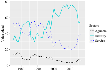
Graph 1. Evolution of value added (% GDP) by sector of activity of the congolese economy. Source: Author, based on World Bank data.
This graph tells us that the industrial sector contributes considerably to the wealth of the country. This is understandable because this sector, which is constituted essentially by extractive industries, is Congo’s first source of income. We can see that since 1975, this sector has consistently increased until 2016. After 2016, there was a decline in the value added of the industrial sector due to the fall in the price of oil. By contrast, the value added of the service sector, which was the first contributor in the 1975s, decreased until 2000. From this date, this sector has experienced a recovery due to its entry in the subregional market of several cell phone companies, banks, and insurance companies. This craze is due to the policy of opening up the state in the 2000s to these various service activities. The agricultural sector has remained rather marginal.
3.4.2. Cameroon
Cameroon’s economy is the locomotive of the subregion, which is a privilege it owes to the dynamic and diversified nature of its economy. Graph 2 shows the evolution of the economy’s sectors of activity.
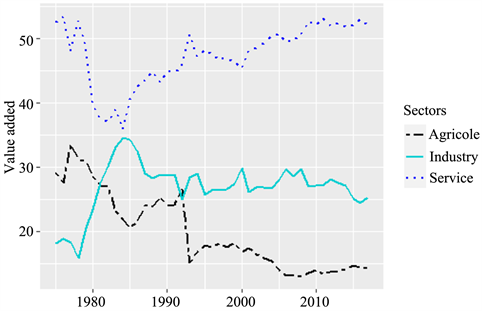
Graph 2. Evolution of value added (% GDP) by sector of activity of the Cameroonian economy. Source: Author, based on World Bank data.
Graph 2 shows that services constitute the primary contribution to the country’s wealth. Since 1975, it can be seen that the value added of the service sector remains well above that of the other sectors. It is followed by the value added of the industrial sector, which makes the second largest contribution to GDP. The value added of the agricultural sector is certainly less important than the that of two previous sectors, but it also contributes to the growth of the country, thus justifying the diversified character of this economy.
In short, examining the evolution of these two economies allows us to see that the value added of the service sector represents the first contribution to national wealth in Cameroon, while in Congo, the value added of the industrial sector is ahead of other sectors. In addition, we note that in Cameroon, all sectors of the economy contribute, in a rather marked way, to GDP, which is not the case for Congo, where only the services and industry sectors are aiming for sustained growth.
4. Presentation and Interpretation of Results
The presentation will be followed by the interpretation of the results.
4.1. Presentation and Analysis of Results
Before running simulations, we performed three preliminary tests: the unit root test, the optimal delay number test and the causality test.
With regard to the unit root test, the results are recorded in Table 3 and show that the variables economic development, agricultural sector, industrial sector and service sector are integrated of order 1. Acceptance of the null hypothesis of the presence of a unit root allows us to conclude that all our variables are stationary in first difference.
![]()
Table 3. Results of stationarity tests.
***significant at 1%; **significant at 5%; *significant at 10%. V_s_agr represents the agricultural sector; V_s_ind represents the industrial sector; V_s_serv represents the service sector; GDP/capita represents economic development. Source: Author’s calculation.
Concerning the optimal number of lags, it emerges from Table 4 that the Akaike and Schwarz criteria all converge for an optimal number of lags equal to one (p* = 1) for these two (2) countries.
![]()
![]()
Table 4. The optimal number of delays.
Source: Author’s calculation.
Furthermore, the results of the causality tests recorded in Table 5(a) and Table 5(b) below show, on the one hand, that the variables for the agricultural,
industrial and service sectors influence economic development, while economic development and the service and industrial sectors have no effect on the agricultural sector. On the other hand, economic development and the industrial sector influence the service sector but not the agricultural sector. Finally, only the service sector influences the industrial sector in the case of Cameroon, while, in Congo, the variables for the agricultural, industrial and service sectors do not influence economic development. However, the variables of economic development and for the service and industrial sectors have an effect on the agricultural sector. Economic development and the industrial and agricultural sectors do not influence the service sector, and economic development and the service and agricultural sectors do not affect the industrial sector.
We also used a few additional tests, including the no autocorrelation test of the residuals and the model stability test, to validate the estimated VAR model. The results of the statistical test for the absence of autocorrelation of residuals recorded in Table 6 and the second-order P-values show that there is an absence of autocorrelation for the residuals. Similarly, the results of the stability test recorded in Table 6 show that the estimated VAR model is stable.
Source: Author’s calculation.
The results of the simulations presented in Table 7 and Table 8 below show the effects of the production sectors on development. As noted agrabove, our analysis will focus on these long-term results, adapted to analyze economic development.
![]()
Table 7. Short-term results of the effects of production sectors on development in Cameroon and Congo.
*Significant at the 10% threshold; Source: Author’s calculation
![]()
Table 8. Long-term results of the impact of production sectors on development in Cameroon and Congo.
*Significant at the 10% threshold; Source: Author’s calculation.
Table 8 shows that the service sector has a positive and significant influence on economic development in both countries at the 1% threshold. Thus, a 1% increase in the value added of the service sector leads to an increase in economic development of 2.980% and 5.586% for Cameroon and Congo, respectively. We note that this increase is greater in Congo than in Cameroon. This result is consistent with the findings of Erumbana et al. (2019), Beqiraja et al. (2019), Vu (2017), and Ghani and O’connel (2016), which all showed that the service sector positively influences economic development.
Furthermore, the results presented in this table show that the agricultural sector negatively and significantly influences economic development in both countries at the 1% threshold. A 1% increase in the value added of the agricultural sector leads to a decrease of −5.471% and −1.699% in economic development in Cameroon and Congo, respectively. However, the industrial sector has a more negative and significant effect on economic development in Cameroon at the threshold of 1%; indeed, a 1% increase in the value added of the industrial sector leads to a −5.400% drop in economic development in Cameroon. These results are close to those of Fagerberg (2000), who examined industries in a sample of 39 countries over the period 1973-1990. He obtained the result that structural change does not contribute to productivity growth or therefore to growth.
The results for the impact of each sector’s long-term impulse responses to shocks on the dynamics of economic development in Congo and Cameroon are recorded in Table 9 and Graph 3.
The reading of these results shows first that economic development reacts positively to innovations in the service sector in both countries. Second, economic development reacts negatively to innovation in the industrial sector in Cameroon. Finally, the reaction of economic development remains ambiguous in both countries following innovations in the agricultural sector, and it remains ambiguous in Congo following innovations in the industrial sector.
Thus, it emerges from this analysis that, in the long term, the service sector contributes positively to economic development and that the industrial and agricultural sectors negatively affect economic development.
![]()
Table 9. Response of economic development to shocks in these three sectors over the long term in Cameroon and Congo.
Source: Author, based on impulse responses.
![]()
(a)
![]()
(b)
Graph 3. Impulse responses. (a) Cameroon’s impulse responses, Source: Author; (b) Congo’s impulse responses, Source: Author.
4.2. Interpretation of Results
Two lessons can be drawn from the results obtained. The first is that the service sector eases development, while the second is that the agricultural and industrial sectors inhibit development.
4.2.1. The Service Sector: A Lubricant for Long-Term Economic Development
Two arguments can justify the service sector’s position as a pillar of economic development: the liberalization of the service sector in the 2000s and the dynamism of the youth of these countries.
Regarding the liberalization of the service sector, the economic opening of these countries has allowed them to develop several service sector industries. Additionally, we see the arrival on the market of new operators that amplify the presence of services in these countries. This entry of newcomers has also allowed the development of south-south trade. Indeed, countries such as South Africa, India and many others are investing heavily in the service sector.
The second reason is the dynamic youth of these countries. By 2050, according to recent United Nations projections, Africa’s population will be among the largest on the planet. In addition, Africa’s population is increasingly in step with new technologies. Thus, an institutional and educational framework adapted to the needs of this population will support the development of the service sectors. Thus, making services a lever for development requires well-qualified population, which the public authorities will be able to offer.
4.2.2. The Agricultural and Industrial Sectors Inhibit Long-Term Economic Development
There are two reasons why the agricultural sector may be slowing economic development: displacements of the population and the lack of attractiveness of the agricultural sector.
With regard to the displacement of the population from rural areas to urban centers, the African Development Report, ADB (2015), notes that currently, the share of rural dwellers in CEMAC is 48.07%, whereas it was 70% in the 1960s. This decline in the rural population finds justification in the poor living conditions of farmers.
Such living conditions have led many young people to leave rural areas to settle in urban areas, with the hope of a better future. This departure of able-bodied youths leaves an old and aging population in rural areas that can no longer find resources to continue or increase production, CEMAC (2004).
With regard to attractiveness, few measures have been taken by public authorities to make the agricultural sector attractive. Indeed, the lack of productivity, probably due to the absence of intensive production methods and new agricultural technologies, could be one of the reasons for this.
For the industrial sector, two arguments can justify these results: the first is that the industrial sector is composed, to a large extent, of the hydrocarbon sector. This sector is an important part of the GDP of countries with oil resources. In Congo, for example, it represents 71.9% of GDP. For some time now, the public authorities, in partnership with private companies, have been struggling to find new oil deposits. This, in the long term, can lead to a scarcity of oil and thus a drop in industrial production.
The second argument that can hinder the growth of industry in these two countries is the “unfavorable business climate”. Gelb et al. (2014), for example, mention, among other impediments, the cost of energy, transportation, corruption, regulation, security, contract enforcement and political instability. For an investor considering developing industrial sector projects in Africa, all these factors undeniably increase the cost of doing business and thus decrease the desire to invest.
5. Conclusion
The objective of this study was to analyze structural change as a factor of economic development in the Economic and Monetary Community of Central Africa (CEMAC). To meet this objective, we used an econometric methodology. In view of the results obtained, we can confirm that the hypothesis presented in this reflection has been confirmed in the service sector. Indeed, the results obtained have shown that in Cameroon and Congo, structural change can take place through the service sector, as it has a positive effect on economic development.
In the new structural economy, the state plays an important role in structural change. This vision of the new structural economy is questionable in its application within CEMAC countries, especially since there are still questions as to whether governments have moved beyond the neoclassical structural and neoliberal approaches to development that recognize the state as benevolent, informed, a leader of change and a buffer against market failures.
The main lesson we have learned from this work is that CEMAC authorities should promote, at the subregional level, policies to facilitate and further develop services, including through public-private partnerships (PPPs). Nevertheless, as in the case of India and in Ruet (2015), the aim should be to develop high value-added service activities with sufficient spillover effects (transport, telecommunications, ICT, banking and financial services, tourism, etc.) on other sectors and to strengthen human capital and productivity.
This development should only take place under the impetus not of a rentier state but rather of a proactive developmental state capable of embodying transformational political leadership and intervening as a strategic state within the framework of state capitalism, as evidenced by the successful experience of the emerging countries of East Asia (Dzaka et al., 2019). At the end of our study, a question remains to be asked, as a research avenue, given that all CEMAC aspire to the status of economic emergence by 2035 (including 2025 for Congo and 2035 for Cameroon). If this emergence implies structural change, and therefore development, is development a credible objective for CEMAC if it skips the stage of the industrialization process that remains, despite everything, at the heart of the economic emergence process today?
This analysis focused on the impact of the production sectors of CEMAC member countries on economic development. In future analyses, we can introduce natural resource rents to assess the impact on economic development.