Perturbation Analysis for the Matrix-Scaled Total Least Squares Problem

Qun Wang, Longyan Li, Pingping Zhang

School of Science, Chongqing University of Posts and Telecommunications, Chongqing, China.

DOI: 10.4236/apm.2021.112008                

Abstract

In this paper, we extend matrix scaled total least squares (MSTLS) problem with a single right-hand side to the case of multiple right-hand sides. Firstly, under some mild conditions, this paper gives an explicit expression of the minimum norm solution of MSTLS problem with multiple right-hand sides. Then, we present the Kronecker-product-based formulae for the normwise, mixed and componentwise condition numbers of the MSTLS problem. For easy estimation, we also exhibit Kronecker-product-free upper bounds for these condition numbers. All these results can reduce to those of the total least squares (TLS) problem which were given by Zheng et al. Finally, two numerical experiments are performed to illustrate our results.

Keywords

Singular Value Decomposition, Matrix-Scaled Total Least Squares, Total Least Squares, Condition Number

1. Introduction

Consider the overdetermined linear system $Ax\approx b$, where $A\in {ℝ}^{m\times n}$ and $b\in {ℝ}^m$, and the total least squares (TLS) problem can be formulated as (see [1] )

$\underset{E\mathrm{,}f}{min}{\Vert \left[\begin{array}{cc}E& f\end{array}\right]\Vert }_F\mathrm{,}\text{subject}\text{to}\left(A+E\right)x=b+f\mathrm{.}$ (1)

However, in many linear parameter estimation problems, the error of data matrix A on the left side of the approximate system may be scaled. In order to maximize the accuracy of the estimated parameters x, the case where the scaling factor is used to weight some columns of error matrix in data matrix A is naturally considered when estimating parameters x using the TLS approach. From the point of view, Liu, Wei and Chen [2] proposed the concept of the matrix-scaled total least squares (MSTLS) problem with single right-hand side in 2019. Inspired by [3], Liu, Wei and Chen [2] transformed the MSTLS problem with single right-hand side into the weighted TLS (WTLS) problem.

As a continuation of their work, we extend the MSTLS problem with single right-hand side to multiple right-hand sides as follows.

$\underset{E\mathrm{,}F}{min}{\Vert \begin{array}{ccc}\gamma E_1& E_2& F\end{array}\Vert }_F\mathrm{,}\text{subject}\text{to}\left(A_1+\gamma E_1\right)X_1+\left(A_2+E_2\right)X_2=B+F\mathrm{,}$ (2)

where $X=\left[\begin{array}{cc}{X}_1& X_2\end{array}\right]\in {ℝ}^{n\times d}$, $A_1\in {ℝ}^{m\times n_1}$, $A_2\in {ℝ}^{m\times n_2}$, $n_1+n_2=n$ and $B\in {ℝ}^{m\times d}\left(m\ge n+d\right)$.

When $d=1$, our model (2) degenerates to the single right-hand case.

The condition number is a measure of the sensitivity of the solution to input data perturbation. Therefore, condition numbers play an important role in numerical analysis. Many scholars have studied the TLS problem with multiple right-hand sides: [4] [5] [6] [7] [8] studied the sufficient conditions or/and necessary conditions for its solvability. When the TLS problem is solvable, Huang, Yan and Yu discussed the solution set and minimal norm solution of the TLS problem, see [4] [9]. Recently, based on singular value decomposition (SVD) of augmented matrix, many scholars have discussed the solution set and minimal norm solution of the TLS problem. In [10], Hnětynková et al. proposed the TLS problem with multiple right-hand sides, and gave the conditions for the existence and expression of the solutions. In [11], Hnětynková et al. extended the concept of the core problem of the TLS problem with single right-hand side proposed by Paige and Strakoš in [12] to the TLS problem with multiple right-hand sides. The perturbation analysis of the solution of the TLS problem with multiple right-hand sides can be found in references [7] [8] [13] [14] [15]. Zheng, Meng and Wei gave the exact expressions and their upper bounds of normwise, mixed and componentwise condition numbers of TLS problem with multiple right-hand sides in [16] [17]. These results extend the condition number theory of TLS problem with single right-hand side. In addition, by making use of the perturbation results in the above references, Liu et al. [18] [19] derived closed formulae for condition numbers of the total least squares problem with linear equality constraint problem.

As far as we know, the perturbation analysis of the MSTLS problem has not been systematically performed in literature. In this paper, we consider the perturbation analysis of the MSTLS problem (2). The relative normwise condition number, the mixed condition number and the componentwise condition number are derived. Our analysis can be seen as a unified treatment of the mentioned approaches in [3] and [16].

Throughout this paper, for given positive integers m and n, we denote by ${ℝ}^{m\times n}$ the space of all $m\times n$ real matrices, and $I_n$ stands for the identity matrix of order n. ${\Vert \cdot \Vert }_2$, ${\Vert \cdot \Vert }_{\infty }$ and ${\Vert \cdot \Vert }_F$ denote the 2-norm, ∞-norm, and Frobenius norm of their arguments, respectively. Given a matrix $X=\left(x_{ij}\right)\in {ℝ}^{m\times n}$, ${\Vert X\Vert }_{max}$, $X^{\text{T}}$, $X^{†}$ and ${\sigma }_i\left(X\right)$ denote the “max” norm given by ${\Vert X\Vert }_{max}=\underset{i\mathrm{,}j}{max}\left|x_{ij}\right|$, the transpose, the Moore-Penrose inverse and the i-th largest singular value of X, respectively. $\left|X\right|$ is the absolute value of the matrix X, whose entries are $\left|x_{ij}\right|$. Moreover, for $Y=\left(y_{ij}\right)$, $Z=\left(z_{ij}\right)\in {ℝ}^{m\times n}$, $\frac{Y}{Z}$ is an entry-wise division; that is, $\frac{Y}{Z}=\left(y_{ij}/z_{ij}\right)$, or Y./Z in Matlab notation. Here, ξ/0 is interpreted as zero if $\xi =0$ and $\infty$ otherwise. For matrices $A=\left[\begin{array}{ccc}{a}_1& \cdots & a_n\end{array}\right]=\left(a_{ij}\right)\in {ℝ}^{m\times n}$, $\text{vec}\left(A\right)={\left[\begin{array}{ccc}{a}_1^{\text{T}}& \cdots & a_n^{\text{T}}\end{array}\right]}^{\text{T}}\in {ℝ}^{mn\times 1}$ and $A\otimes B=\left[a_{ij}B\right]$ denotes the Kronecker product of A and any matrix B. Let ${\Pi }_{\left(m,n\right)}={\displaystyle {\sum }_{i=1}^m}{\displaystyle {\sum }_{j=1}^n}{E}_{ij}\otimes E_{ij}^{\text{T}}$, where $E_{ij}\in {ℝ}^{m\times n}$ has an entry 1 in position $\left(i\mathrm{,}j\right)$ and all other entries are zeros.

The organization of this paper is as follows. In Section 2, we present some necessary preliminaries, including the explicit expression for minimum $W_{\gamma }^{-2}$ -norm MSTLS solution under some mild conditions and some important lemmas. In Section 3, we derive the normwise, mixed and componentwise condition numbers and their computable upper bounds of the MSTLS solution. All these results can reduce to those of the TLS problem which were given in [16]. Two numerical examples are tested in Section 4 to demonstrate the tightness of the derived upper bounds. Some concluding remarks are given in Section 5. In the appendix, we present a power method for calculating the normwise condition number of the MSTLS solution $X_{\text{MSTLS}}$ similar to the one in [20].

2. Preliminaries

In this section, we give an explicit expression for the minimum $W_{\gamma }^{-2}$ -norm solution of the MSTLS problem with multiple right-hand sides (2) under some mild conditions.

Along the similar lines as in [2] [3], we can see that (2) is equivalent to the following WTLS model:

$\underset{E\mathrm{,}F}{min}{\Vert \left[\begin{array}{ccc}{E}_1& E_2& F\end{array}\right]\Vert }_F\mathrm{,}\text{subject}\text{to}\left[\left(\gamma A_1\mathrm{,}{A}_2\right)+\left(E_1\mathrm{,}{E}_2\right)\right]W_{\gamma }^{-1}X=B+F\mathrm{,}$ (3)

where $W_{\gamma }=\left[\begin{array}{cc}\gamma I_{n_1}& 0\\ 0& I_{n_2}\end{array}\right]$. Let

$A_{\gamma }=\left[\begin{array}{cc}A& B\end{array}\right]{\bar{W}}_{\gamma }\text{with}{\bar{W}}_{\gamma }=\left[\begin{array}{cc}{W}_{\gamma }& 0\\ 0& I_d\end{array}\right]\mathrm{,}$

and the SVD of $A_{\gamma }$ be

$A_{\gamma }=U\Sigma V^{\text{T}}=\left[\begin{array}{cc}{U}_1& U_2\end{array}\right]\left[\begin{array}{cc}{\Sigma }_1& 0\\ 0& {\Sigma }_2\end{array}\right]\left[\begin{array}{c}{V}_1^{\text{T}}\\ V_2^{\text{T}}\end{array}\right]\mathrm{,}$ (4)

where $U_1\in {ℝ}^{m\times p}$, $U_2\in {ℝ}^{m\times \left(m-p\right)}$, $V_1=\begin{array}{c}n\\ d\end{array}\left[\begin{array}{c}{V}_{11}\\ V_{21}\end{array}\right]\in {ℝ}^{\left(n+d\right)\times p}$, $V_2=\begin{array}{c}n\\ d\end{array}\left[\begin{array}{c}{V}_{12}\\ V_{22}\end{array}\right]\in {ℝ}^{\left(n+d\right)\times \left(n+d-p\right)}$, ${\Sigma }_1=\text{diag}\left({\sigma }_1\mathrm{,}{\sigma }_2\mathrm{,}\cdots \mathrm{,}{\sigma }_p\right)\in {ℝ}^{p\times p}$ and ${\Sigma }_2=\text{diag}\left({\sigma }_{p+1}\mathrm{,}{\sigma }_{p+2}\mathrm{,}\cdots \mathrm{,}{\sigma }_{n+d}\right)\in {ℝ}^{\left(m-p\right)\times \left(n+d-p\right)}$.

The following theorem gives the minimum $W_{\gamma }^{-2}$ -norm solution of (2).

Theorem 2.1 Let the SVD of $A_{\gamma }$ be given as in (4). If

$p\le n\mathrm{,}{\sigma }_p>{\sigma }_{p+1}\text{and}\text{rank}\left(V_{22}\right)=d\mathrm{,}$ (5)

thenthe MSTLS problem with multiple right-hand sides (2) has the minimum $W_{\gamma }^{-2}$ -norm solution:

$X_{\text{MSTLS}}=-W_{\gamma }{V}_{12}{V}_{22}^{†}\mathrm{,}$ (6)

wherethe weighted $W_{\gamma }^{-2}$ -norm is defined by ${\Vert X\Vert }_{W_{\gamma }^{-2}}=\sqrt{\text{trace}\left(X^{\text{T}}{W}_{\gamma }^{-2}X\right)}$.

Proof. By ( [8], (2.3)), we can get the minimum F-norm solution to (3) under the condition (5):

$W_{\gamma }^{-1}{X}_{\text{MSTLS}}=-V_{12}{V}_{22}^{†}\mathrm{,}$

which leads to the minimum $W_{\gamma }^{-2}$ -norm solution of (2)

$X_{\text{MSTLS}}=-W_{\gamma }{V}_{12}{V}_{22}^{†}\mathrm{.}$

Therefore, we complete the proof.

In this paper, all discussions are based on the solvability conditions (5). Next we give some lemmas which will be used in the next analysis.

Lemma 2.1 ( [21], Chapt. 2) Let $B\in {ℝ}^{m\times n}$ , $C\in {ℝ}^{p\times q}$ , $X\in {ℝ}^{n\times p}$ . Then

${\left(B\otimes C\right)}^{\text{T}}=B^{\text{T}}\otimes C^{\text{T}}\mathrm{,}{\Vert B\otimes C\Vert }_2={\Vert B\Vert }_2{\Vert C\Vert }_2\mathrm{,}$

$\text{vec}\left(BXC\right)=\left(C^{\text{T}}\otimes B\right)\text{vec}\left(X\right)\mathrm{,}$

$\text{vec}\left(B^{\text{T}}\right)={\Pi }_{\left(m\mathrm{,}n\right)}\text{vec}\left(B\right)\mathrm{,}$

${\Pi }_{\left(p\mathrm{,}m\right)}\left(C\otimes B\right)=\left(B\otimes C\right){\Pi }_{\left(n\mathrm{,}q\right)}\mathrm{.}$

If an orthogonal matrix of size n is partitioned into a $2\times 2$ block form, some interesting connections and properties among these four submatrix blocks are provided in the lemma below.

Lemma 2.2 ( [16], Lemma 2.1) Let $Q=\left[\begin{array}{cc}{Q}_{11}& Q_{12}\\ Q_{21}& Q_{22}\end{array}\right]$ be an n-by-n orthogonal matrix with a 2-by-2 partitioning. Then

1) $Q_{11}$ has full column (row)rank if and only if $Q_{22}$ has full row (column) rank;

2) ${\Vert Q_{11}^{†}\Vert }_2={\Vert Q_{22}^{†}\Vert }_2$, ${\left(Q_{11}^{\text{T}}\right)}^{†}=Q_{11}-Q_{12}{Q}_{22}^{†}{Q}_{21}$, ${\left(Q_{11}^{\text{T}}\right)}^{†}{Q}_{21}^{\text{T}}=-Q_{12}{Q}_{22}^{†}$.

Since the MSTLS solution is closely related to the matrix V of right singular vectors of augmented matrix, the first-order perturbation analysis of V will play an important role in next discussions. The next lemma gives the first-order perturbation analysis of V.

Lemma 2.3 ( [16], Lemma 2.2) Let $A_{\gamma }$ have the SVD in (4) with ${\sigma }_p>{\sigma }_{p+1}$ and ${\Vert E\Vert }_2$ be sufficiently small. Define

$R\mathrm{<mo>\; =\; </mo>}{\left({\Sigma }_1^2\otimes I_{n+d-p}-I_p\otimes \left({\Sigma }_2^{\text{T}}{\Sigma }_2\right)\right)}^{-1}\left[\begin{array}{cc}{I}_p\otimes {\Sigma }_2^{\text{T}}& {\Sigma }_1\otimes I_{n+d-p}\end{array}\right]\mathrm{,}$

$S=\left[\begin{array}{c}{V}_1^{\text{T}}\otimes U_2^{\text{T}}\\ {\Pi }_{\left(p\mathrm{,}n+d-p\right)}\left(V_2^{\text{T}}\otimes U_1^{\text{T}}\right)\end{array}\right]\mathrm{.}$

Then the matrix $\tilde{V}=\left[\begin{array}{cc}{\tilde{V}}_1& {\tilde{V}}_2\end{array}\right]$ of right singular vectors of ${\tilde{A}}_{\gamma }=A_{\gamma }+E$ satisfies

${\tilde{V}}_1=\left(V_1+V_{2}P\right){\left(I+P^{\text{T}}P\right)}^{-\frac{1}{2}}\mathrm{,}{\tilde{V}}_2=\left(V_2-V_1{P}^{\text{T}}\right){\left(I+P{P}^{\text{T}}\right)}^{-\frac{1}{2}}\mathrm{,}$

where $P\in {ℝ}^{\left(n+d-p\right)\times p}$ is given by

$\text{vec}\left(P\right)=RS\text{vec}\left(E\right)+\mathcal{O}\left({\Vert E\Vert }_2^2\right)\mathrm{.}$

Moreover, if $V_{22}$ has full row (column)rank,then ${\tilde{V}}_{22}$ has full row (column) rank.

3. Condition Numbers of X_MSTLS

Let $\tilde{A}=\left[\begin{array}{cc}{\tilde{A}}_1& {\tilde{A}}_2\end{array}\right]=A+\Delta A$ and $\tilde{B}=B+\Delta B$, where $\Delta A=\left[\begin{array}{cc}\Delta A_1& \Delta A_2\end{array}\right]$ and $\Delta B$ are the perturbations of the input data A and B, respectively.

Consider the perturbed MSTLS problem with multiple right-hand sides

$\underset{E\mathrm{,}F}{min}{\Vert \left(\begin{array}{ccc}\gamma E_1& E_2& F\end{array}\right)\Vert }_F\mathrm{,}\text{subject}\text{to}\left({\tilde{A}}_1+\gamma E_1\right)X_1+\left({\tilde{A}}_2+E_2\right)X_2=\tilde{B}+F\mathrm{.}$ (7)

Similarly, (7) is also treated as a perturbed WTLS problem. Let ${\tilde{A}}_{\gamma }=\left[\begin{array}{cc}\tilde{A}& \tilde{B}\end{array}\right]{\bar{W}}_{\gamma }$, and the SVD of ${\tilde{A}}_{\gamma }$ be

${\tilde{A}}_{\gamma }=\tilde{U}\tilde{\Sigma }{\tilde{V}}^{\text{T}}=\left[\begin{array}{cc}{\tilde{U}}_1& {\tilde{U}}_2\end{array}\right]\left[\begin{array}{cc}{\tilde{\Sigma }}_1& 0\\ 0& {\tilde{\Sigma }}_2\end{array}\right]{\left[\begin{array}{cc}{\tilde{V}}_{11}& {\tilde{V}}_{12}\\ {\tilde{V}}_{21}& {\tilde{V}}_{22}\end{array}\right]}^{\text{T}}\mathrm{,}$ (8)

where $\tilde{U}$, $\tilde{\Sigma }$ and $\tilde{V}$ are partitioned as in U, $\Sigma$ and V in (4), respectively.

When the norm ${\Vert \left[\begin{array}{cc}\Delta A& \Delta B\end{array}\right]\Vert }_F$ of the perturbations is sufficiently small, then perturbation analysis of singular values can ensure that the perturbed MSTLS problem with multiple right-hand sides (7) has the minimum $W_{\gamma }^{-2}$ -norm solution:

${\tilde{X}}_{\text{MSTLS}}=-W_{\gamma }{\tilde{V}}_{12}{\tilde{V}}_{22}^{†}\mathrm{.}$ (9)

Let $\Delta X={\tilde{X}}_{\text{MSTLS}}-X_{\text{MSTLS}}$. Now we introduce definitions of the normwise, mixed and componentwise condition numbers for $X_{\text{MSTLS}}$ as follows.

Definition 3.1 The absolute normwise condition number for $X_{\text{MSTLS}}$ is defined by

${\kappa }_{\text{MSTLS}}^{\text{abs}}\left(X_{\text{MSTLS}}\mathrm{,}{A}_{\gamma }\right)\mathrm{<mo>\; :\; </mo>}=\underset{\epsilon \to 0}{lim}\underset{{\Vert \Delta A_{\gamma }\Vert }_F\le \epsilon {\Vert A_{\gamma }\Vert }_F}{lim}\frac{{\Vert \Delta X\Vert }_F}{{\Vert \Delta A_{\gamma }\Vert }_F}\mathrm{,}$ (10)

therelative normwise condition number for $X_{\text{MSTLS}}$ is defined by

${\kappa }_{\text{MSTLS}}^{\text{rel}}\left(X_{\text{MSTLS}}\mathrm{,}{A}_{\gamma }\right)\mathrm{<mo>\; :\; </mo>}=\underset{\epsilon \to 0}{lim}\underset{{\Vert \Delta A_{\gamma }\Vert }_F\le \epsilon {\Vert A_{\gamma }\Vert }_F}{lim}\frac{{\Vert \Delta X\Vert }_F}{\epsilon {\Vert X_{\text{MSTLS}}\Vert }_F}\mathrm{,}$ (11)

themixed condition number for $X_{\text{MSTLS}}$ is defined by

${\kappa }_{\text{MSTLS}}^{\text{mix}}\left(X_{\text{MSTLS}}\mathrm{,}{A}_{\gamma }\right)\mathrm{<mo>\; :\; </mo>}=\underset{\epsilon \to 0}{lim}\underset{\begin{array}{c}\left|\Delta A{W}_{\gamma }\right|\le \epsilon \left|A{W}_{\gamma }\right|\\ \left|\Delta B\right|\le \epsilon \left|B\right|\end{array}}{sup}\frac{{\Vert \Delta X\Vert }_{max}}{\epsilon {\Vert X_{\text{MSTLS}}\Vert }_{max}}\mathrm{,}$ (12)

andthe componentwise condition number for $X_{\text{MSTLS}}$ is defined by

${\kappa }_{\text{MSTLS}}^{\text{com}}\left(X_{\text{MSTLS}}\mathrm{,}{A}_{\gamma }\right)\mathrm{<mo>\; :\; </mo>}=\underset{\epsilon \to 0}{lim}\underset{\begin{array}{c}\left|\Delta A{W}_{\gamma }\right|\le \epsilon \left|A{W}_{\gamma }\right|\\ \left|\Delta B\right|\le \epsilon \left|B\right|\end{array}}{sup}\frac{1}{\epsilon }{\Vert \frac{\Delta X}{X_{\text{MSTLS}}}\Vert }_{max}\mathrm{.}$ (13)

Definition 3.1 only provides general descriptions of the various condition numbers. It is usually hard to give their exact computable formulae. However, if $X_{\text{MSTLS}}$ is a differentiable function with respect to the data, the condition numbers defined in Definition 3.1 can be exactly expressed in derivatives. We start from the differentiability of $X_{\text{MSTLS}}$.

Let the SVD of the matrices $A_{\gamma }$ be given as in (4). To derive the exact formulae of the condition numbers of $X_{\text{MSTLS}}=-W_{\gamma }{V}_{12}{V}_{22}^{†}$, we define the mapping $\varphi \mathrm{<mo>\; :\; </mo>}{ℝ}^{m\left(n+d\right)}\to {ℝ}^{nd}$ by

$\varphi \left(c\right)=\text{vec}\left(X_{\text{MSTLS}}\right)\mathrm{,}$

where $c=\text{vec}\left(A_{\gamma }\right)$. It follows from Lemma 2.3 that $\varphi$ is continuous in a neighborhood of c. Using the definitions of the condition numbers of the mapping $\varphi$ at a fixed point c [22] [23] [24], and following [23] [24] [25], if $\varphi$ is Fréchet differentiable in a neighborhood of c, we have

${\kappa }_{\text{MSTLS}}^{\text{abs}}\left(X_{\text{MSTLS}}\mathrm{,}{A}_{\gamma }\right)={\kappa }_{\text{MSTLS}}^{\text{abs}}\left(\varphi \mathrm{,}c\right)={\Vert {\varphi }^{\prime }\left(c\right)\Vert }_2\mathrm{,}$ (14)

${\kappa }_{\text{MSTLS}}^{\text{rel}}\left(X_{\text{MSTLS}}\mathrm{,}{A}_{\gamma }\right)={\kappa }_{\text{MSTLS}}^{\text{rel}}\left(\varphi \mathrm{,}c\right)=\frac{{\Vert {\varphi }^{\prime }\left(c\right)\Vert }_2{\Vert c\Vert }_2}{{\Vert \varphi \left(c\right)\Vert }_2}\mathrm{,}$ (15)

${\kappa }_{\text{MSTLS}}^{\text{mix}}\left(X_{\text{MSTLS}}\mathrm{,}{A}_{\gamma }\right)={\kappa }_{\text{MSTLS}}^{\text{mix}}\left(\varphi \mathrm{,}c\right)=\frac{{\Vert \left|{\varphi }^{\prime }\left(c\right)\right|\left|c\right|\Vert }_{\infty }}{{\Vert \varphi \left(c\right)\Vert }_{\infty }}\mathrm{,}$ (16)

${\kappa }_{\text{MSTLS}}^{\text{com}}\left(X_{\text{MSTLS}}\mathrm{,}{A}_{\gamma }\right)={\kappa }_{\text{MSTLS}}^{\text{com}}\left(\varphi \mathrm{,}c\right)={\Vert \frac{\left|{\varphi }^{\prime }\left(c\right)\right|\left|c\right|}{\left|\varphi \left(c\right)\right|}\Vert }_{\infty }\mathrm{,}$ (17)

where ${\varphi }^{\prime }\left(c\right)$ denotes the Fréchet derivative of $\varphi$ at point c.

Before deriving the explicit expression for condition numbers, we give a useful lemma which proves that $\varphi$ is Fréchet differentiable in a neighborhood of $c=\text{vec}\left(A_{\gamma }\right)$ and gives the explicit expression for ${\varphi }^{\prime }\left(c\right)$.

Lemma 3.1 Under conditions (5), the mapping $\varphi$ defined above is continuous and Fréchet differentiable at $c=\text{vec}\left(A_{\gamma }\right)$ . Moreover, its Fréchet derivative has the expression

${\varphi }^{\prime }\left(c\right)=\left(H_1+H_2\right)RS$ (18)

inwhich R and S are defined as in Lemma 2.3,and

$H_1=\left({\left(V_{22}{V}_{22}^{\text{T}}\right)}^{-1}{V}_{21}\right)\otimes \left(W_{\gamma }{V}_{12}{F}_{V_{22}}\right)\mathrm{,}{H}_2=\left({\left(V_{22}^{†}\right)}^{\text{T}}\otimes W_{\gamma }{\left(V_{11}^{\text{T}}\right)}^{†}\right){\Pi }_{\left(n+d-p\mathrm{,}p\right)}$

with $F_{V_{22}}=I-V_{22}^{†}{V}_{22}$.

Proof. We only prove the second statement since the first part is trivial. According to Lemma 2.3, it follows that there exists a proper matrix P such that

${\tilde{V}}_{12}=\left(V_{12}-V_{11}{P}^{\text{T}}\right){\left(I+P{P}^{\text{T}}\right)}^{-\frac{1}{2}}\mathrm{,}{\tilde{V}}_{22}=\left(V_{22}-V_{21}{P}^{\text{T}}\right){\left(I+P{P}^{\text{T}}\right)}^{-\frac{1}{2}}\mathrm{.}$

Since ${\tilde{V}}_{22}$ has full row rank by Lemma 2.3, we have

$\begin{array}{c}{\tilde{X}}_{\text{MSTLS}}=-W_{\gamma }{\tilde{V}}_{12}{\tilde{V}}_{22}^{†}=-W_{\gamma }{\tilde{V}}_{12}{\tilde{V}}_{22}^{\text{T}}{\left({\tilde{V}}_{22}{\tilde{V}}_{22}^{\text{T}}\right)}^{-1}\\ =-W_{\gamma }\left(V_{12}-V_{11}{P}^{\text{T}}\right){\left(I+P{P}^{\text{T}}\right)}^{-1}{\left(V_{22}-V_{21}{P}^{\text{T}}\right)}^{\text{T}}\\ \times {\left(\left(V_{22}-V_{21}{P}^{\text{T}}\right){\left(I+P{P}^{\text{T}}\right)}^{-1}{\left(V_{22}-V_{21}{P}^{\text{T}}\right)}^{\text{T}}\right)}^{-1}\mathrm{.}\end{array}$

Using Lemma 2.2 and only retaining the first-order terms give

$\begin{array}{c}{\tilde{X}}_{\text{MSTLS}}=X_{\text{MSTLS}}+W_{\gamma }{V}_{12}\left(I-V_{22}^{†}{V}_{22}\right)P{V}_{21}^{\text{T}}{\left(V_{22}{V}_{22}^{\text{T}}\right)}^{-1}\\ +W_{\gamma }\left(V_{11}-V_{12}{V}_{22}^{†}{V}_{21}\right)P^{\text{T}}{V}_{22}^{†}+\mathcal{O}\left({\Vert \Delta A_{\gamma }\Vert }_2^2\right)\\ =X_{\text{MSTLS}}+W_{\gamma }{V}_{12}{F}_{V_{22}}P{V}_{21}^{\text{T}}{\left(V_{22}{V}_{22}^{\text{T}}\right)}^{-1}\\ +W_{\gamma }{\left(V_{11}^{\text{T}}\right)}^{†}{P}^{\text{T}}{V}_{22}^{†}+\mathcal{O}\left({\Vert \Delta A_{\gamma }\Vert }_2^2\right)\mathrm{,}\end{array}$

which together with Lemma 2.1 and Lemma 2.3 leads to

$\begin{array}{l}\varphi \left(\text{vec}\left({\tilde{A}}_{\gamma }\right)\right)-\varphi \left(\text{vec}\left(A_{\gamma }\right)\right)\\ =\text{vec}\left({\tilde{X}}_{\text{MSTLS}}-X_{\text{MSTLS}}\right)\\ =(\left({\left(V_{22}{V}_{22}^{\text{T}}\right)}^{-1}{V}_{21}\right)\otimes \left(W_{\gamma }{V}_{12}{F}_{V_{22}}\right)\\ +\left({\left(V_{22}^{†}\right)}^{\text{T}}\otimes W_{\gamma }{\left(V_{11}^{\text{T}}\right)}^{†}\right){\Pi }_{\left(n+d-p\mathrm{,}p\right)})\text{vec}\left(P\right)+\mathcal{O}\left({\Vert \Delta A_{\gamma }\Vert }_2^2\right)\\ =\left(H_1+H_2\right)RS\text{vec}\left(\Delta A_{\gamma }\right)+\mathcal{O}\left({\Vert \Delta A_{\gamma }\Vert }_2^2\right)\mathrm{.}\end{array}$

Consequently, the Fréchet derivative of $\varphi$ at $c={\left[\begin{array}{cc}{a}^{\text{T}}& b^{\text{T}}\end{array}\right]}^{\text{T}}$ is given by

${\varphi }^{\prime }\left(c\right)=\left(H_1+H_2\right)RS\mathrm{,}$

which gives the desired result.

3.1. Normwise Condition Numbers

Next, we present the absolute and relative normwise condition numbers of $X_{\text{MSTLS}}$.

Theorem 3.1 Let R be defined as in Lemma 2.3, and $H_1,H_2$ be defined as in Lemma 3.1. Under conditions (5), we have

${\kappa }_{\text{MSTLS}}^{\text{abs}}={\Vert \left(H_1+H_2\right)R\Vert }_2\mathrm{,}$ (19)

${\kappa }_{\text{MSTLS}}^{\text{rel}}=\frac{{\Vert \left(H_1+H_2\right)R\Vert }_2{\Vert A_{\gamma }\Vert }_F}{{\Vert X_{\text{MSTLS}}\Vert }_F}\mathrm{.}$ (20)

Proof. By (14), (15), Lemma 3.1 and the fact that $S{S}^{\text{T}}=I_{n\left(m+d-n\right)}$, the desired results are easily obtained.

Remark 3.1 Taking $\gamma =1$ , our results in (19) and (20) reduce to those of the solution to TLS problem with multiple right-hand sides in ( [16], Theorem 3.3), respectively.

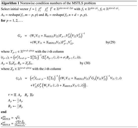
Computing ${\kappa }_{\text{MSTLS}}^{\text{abs}}$ and ${\kappa }_{\text{MSTLS}}^{\text{rel}}$ reduces to computing the spectral norm of matrix $\left(H_1+H_2\right)R$. It should be noted that the Kronecker product enlarges the size of the matrix when m and n are large, so it impossible to explicitly form and store the high dimensions matrix. Along the similar lines as in ( [26], Algorithm 1), we also adopt the iterative technique based on the power method ( [27], p. 289) to eliminate the influence of the Kronecker product. We include it as an appendix.

In many applications, an upper bound would be sufficient to estimate the normwise condition number of the MSTLS solution. We next present the upper bounds for ${\kappa }_{\text{MSTLS}}^{\text{abs}}$ and ${\kappa }_{\text{MSTLS}}^{\text{rel}}$, which only involve the singular values ${\sigma }_p$ and ${\sigma }_{p+1}$ of $A_{\gamma }$. Such bounds are particularly appealing for large-scale MSTLS problem.

Theorem 3.2 Using the notation above, we have the upper bounds for the absolute and relative normwise condition numbers of $X_{\text{MSTLS}}$ as follows:

${\kappa }_{\text{MSTLS}}^{\text{abs}}\le \left(1+{\Vert X_{\text{MSTLS}}\Vert }_2^2\right){\Vert W_{\gamma }\Vert }_2\frac{\sqrt{{\sigma }_p^2+{\sigma }_{p+1}^2}}{{\sigma }_p^2-{\sigma }_{p+1}^2}\mathrm{<mo>\; :\; </mo>}={\bar{\kappa }}_{\text{MSTLS}}^{\text{abs}}\mathrm{,}$ (21)

and

${\kappa }_{\text{MSTLS}}^{\text{rel}}\le \left(1+{\Vert X_{\text{MSTLS}}\Vert }_2^2\right){\Vert W_{\gamma }\Vert }_2\frac{\sqrt{{\sigma }_p^2+{\sigma }_{p+1}^2}}{{\sigma }_p^2-{\sigma }_{p+1}^2}\frac{{\Vert A_{\gamma }\Vert }_F}{{\Vert X_{\text{MSTLS}}\Vert }_F}\mathrm{<mo>\; :\; </mo>}={\bar{\kappa }}_{\text{MSTLS}}^{\text{rel}}\mathrm{,}$ (22)

where ${\sigma }_p$ and ${\sigma }_{p+1}$ are singular values of $A_{\gamma }$.

Proof. According to Lemma 2.1 and Theorem 3.1, we use the CS decomposition ( [28], Theorem 2.6.3) and the property of 2-norm to follow a path similar to the proof in ( [16], Theorem 3.6), the corresponding results can be proved.

Remark 3.2 Taking $\gamma =1$ , our result (21) reduces to that of the TLS problem with multiple right-hand sides in ( [16], Theorem 3.6).

Note that $V_{22}^{\text{T}}\in {ℝ}^{n+1-p}$ and $V_{22}^{†}=\frac{V_{22}^{\text{T}}}{{\Vert V_{22}\Vert }_2^2}$ when $d=1$, and we can get the following corollary about the normwise condition numbers and their upper bounds for the MSTLS problem with single right-hand side by Theorems 3.1 and 3.2.

Corollary 3.1 Consider the MSTLS problem with single-hand side, if ${\sigma }_p>{\sigma }_{p+1}$ and $V_{22}\ne 0$ , we have

$\begin{array}{c}{\kappa }_{\text{MSTLS}}^{\text{abs}}=\frac{1}{{\Vert V_{22}\Vert }_2^2}{\Vert \left(V_{21}\otimes \left(W_{\gamma }{V}_{12}+x{V}_{22}\right)+\left(W_{\gamma }{V}_{11}+x{V}_{21}\right)\otimes V_{22}\right)R\Vert }_2\\ \le \left(1+{\Vert x\Vert }_2^2\right){\Vert W_{\gamma }\Vert }_2\frac{\sqrt{{\sigma }_p^2+{\sigma }_{p+1}^2}}{{\sigma }_p^2-{\sigma }_{p+1}^2}\mathrm{<mo>\; :\; </mo>}={\bar{\kappa }}_{\text{MSTLS}}^{\text{abs}}\mathrm{,}\end{array}$ (23)

and

$\begin{array}{c}{\kappa }_{\text{MSTLS}}^{\text{rel}}=\frac{{\Vert \left(V_{21}\otimes \left(W_{\gamma }{V}_{12}+x{V}_{22}\right)+\left(W_{\gamma }{V}_{11}+x{V}_{21}\right)\otimes V_{22}\right)R\Vert }_2{\Vert A_{\gamma }\Vert }_F}{{\Vert V_{22}\Vert }_2^2{\Vert x\Vert }_F}\\ \le \left(1+{\Vert x\Vert }_2^2\right){\Vert W_{\gamma }\Vert }_2\frac{\sqrt{{\sigma }_p^2+{\sigma }_{p+1}^2}}{{\sigma }_p^2-{\sigma }_{p+1}^2}\frac{{\Vert A_{\gamma }\Vert }_F}{{\Vert x\Vert }_F}\mathrm{<mo>\; :\; </mo>}={\bar{\kappa }}_{\text{MSTLS}}^{\text{rel}}\mathrm{,}\end{array}$ (24)

wherex is the minimum $W_{\gamma }^2$ -norm solution of the MSTLS problem with single right-hand side.

Remark 3.3 Taking $\gamma =1$ , our results in (23) reduce to those of the TLS problem with single right-hand side in ( [16], Corollaries 3.4 and 3.8).

3.2. Mixed and Componentwise Condition Numbers

When the data are badly scaled and sparse, normwise condition numbers allow large relative perturbations on small entries and may give overestimated bounds. Instead of measuring perturbations by norms, a componentwise condition number is more suitable because it measures perturbation errors for each component of the input data [24]. Therefore, the mixed, componentwise condition numbers for the MSTLS problem are worth studying. In the following theorem, we present the mixed and componentwise condition numbers of the MSTLS problem.

Theorem 3.3 Using the notation above, we have the mixed and componentwise condition numbers of the MSTLS solution as follows:

${\kappa }_{\text{MSTLS}}^{\text{mix}}=\frac{{\Vert \left|KN\right|\text{vec}\left(\left[\begin{array}{cc}\left|A{W}_{\gamma }\right|& \left|B\right|\end{array}\right]\right)\Vert }_{\infty }}{{\Vert X_{\text{MSTLS}}\Vert }_{max}}\mathrm{,}$ (25)

and

${\kappa }_{\text{MSTLS}}^{\text{com}}={\Vert \frac{\left|KN\right|\text{vec}\left(\left[\begin{array}{cc}\left|A{W}_{\gamma }\right|& \left|B\right|\end{array}\right]\right)}{\text{vec}\left(X_{\text{MSTLS}}\right)}\Vert }_{\infty }\mathrm{,}$ (26)

where

$K=\left(H_1+H_2\right){\left({\Sigma }_1^2\otimes I_{n+d-p}-I_p\otimes \left({\Sigma }_2^{\text{T}}{\Sigma }_2\right)\right)}^{-1}\mathrm{,}$

$N=V_1^{\text{T}}\otimes \left({\Sigma }_2^{\text{T}}{U}_2^{\text{T}}\right)+{\Pi }_{\left(n+d-p\mathrm{,}p\right)}\left(V_2^{\text{T}}\otimes \left({\Sigma }_1{U}_1^{\text{T}}\right)\right)\mathrm{.}$

Proof. The proof can easily be obtained by (16), (17) and Lemma 3.1, so we omit it here.

Remark 3.4 Taking $\gamma =1$ , our results in Theorem 3.3 reduce to those of the TLS problem with multiple right-hand sides in ( [16], Theorem 3.11).

The expressions of the condition numbers in Theorem 3.3 involve permutation matrix ${\Pi }_{\left(n+d-p\mathrm{,}p\right)}$ (or ${\Pi }_{\left(p\mathrm{,}n+d-p\right)}$ ) and extensive computation of Kronecker products, so it is not easy to use these expressions to calculate the condition number directly, which is impractical for large-scale problem. Similarly, we also give upper bounds for the mixed and componentwise condition numbers of the MSTLS problem, respectively.

Theorem 3.4 Using the notation above, we have the upper bounds for the mixed and componentwise condition numbers of the MSTLS solution as follows:

${\kappa }_{\text{MSTLS}}^{\text{mix}}\le \frac{{\Vert \left|W_{\gamma }{\left(V_{11}^{\text{T}}\right)}^{†}\right|{\hat{K}}^{\text{T}}\left|V_{22}^{†}\right|+\left|W_{\gamma }{V}_{12}{F}_{V_{22}}\right|\hat{K}\left|V_{21}^{\text{T}}{\left(V_{22}{V}_{22}^{\text{T}}\right)}^{-1}\right|\Vert }_{max}}{{\Vert X_{\text{MSTLS}}\Vert }_{max}}=\mathrm{<mo>\; :\; </mo>}{\bar{\kappa }}_{\text{MSTLS}}^{\text{mix}}\mathrm{,}$ (27)

${\kappa }_{\text{MSTLS}}^{\text{com}}\le {\Vert \frac{\left|W_{\gamma }{\left(V_{11}^{\text{T}}\right)}^{†}\right|{\hat{K}}^{\text{T}}\left|V_{22}^{†}\right|+\left|W_{\gamma }{V}_{12}{F}_{V_{22}}\right|\hat{K}\left|V_{21}^{\text{T}}{\left(V_{22}{V}_{22}^{\text{T}}\right)}^{-1}\right|}{X_{\text{MSTLS}}}\Vert }_{max}=\mathrm{<mo>\; :\; </mo>}{\bar{\kappa }}_{\text{MSTLS}}^{\text{com}}\mathrm{,}$ (28)

where $\hat{K}\in {ℝ}^{\left(n+d-p\right)\times p}$ has the i-th column

$\begin{array}{l}{\hat{k}}_i={\left({\sigma }_i^2{I}_{n+d-p}-{\Sigma }_2^{\text{T}}{\Sigma }_2\right)}^{-1}(\left|{\Sigma }_2^{\text{T}}{U}_2^{\text{T}}\right|\left[\begin{array}{cc}\left|A{W}_{\gamma }\right|& \left|B\right|\end{array}\right]\left|V_1\right|\\ +\left|V_2^{\text{T}}\right|{\left[\begin{array}{cc}\left|A{W}_{\gamma }\right|& \left|B\right|\end{array}\right]}^{\text{T}}\left|U_1{\Sigma }_1\right|)e_i\mathrm{.}\end{array}$

Proof. According to Theorem 3.3 and Lemma 2.1, we have

$\begin{array}{l}\left|KN\right|\text{vec}\left(\left[\begin{array}{cc}\left|A{W}_{\gamma }\right|& \left|B\right|\end{array}\right]\right)\\ \le \left|K\right|\left(\left|V_1^{\text{T}}\right|\otimes \left|{\Sigma }_2^{\text{T}}{U}_2^{\text{T}}\right|+{\Pi }_{\left(n+d-p\mathrm{,}p\right)}\left(\left|V_2^{\text{T}}\right|\otimes \left|{\Sigma }_1{U}_1^{\text{T}}\right|\right)\right)\times \text{vec}\left(\left[\begin{array}{cc}\left|A{W}_{\gamma }\right|& \left|B\right|\end{array}\right]\right)\\ =\left|H_1+H_2\right|{\left({\Sigma }_1^2\otimes I_{n+d-p}-{\sigma }_{p+1}^2{I}_{p\left(n+d-p\right)}\right)}^{-1}\\ \times \text{vec}\left(\left|{\Sigma }_2^{\text{T}}{U}_2^{\text{T}}\right|\left[\begin{array}{cc}\left|A{W}_{\gamma }\right|& \left|B\right|\end{array}\right]\left|V_1\right|+\left|V_2^{\text{T}}\right|{\left[\begin{array}{cc}\left|A{W}_{\gamma }\right|& \left|B\right|\end{array}\right]}^{\text{T}}\left|U_1{\Sigma }_1\right|\right)\text{vec}\left(\left[\begin{array}{cc}\left|A{W}_{\gamma }\right|& \left|B\right|\end{array}\right]\right)\\ =\left|\left({\left(V_{22}^{†}\right)}^{\text{T}}\otimes W_{\gamma }{\left(V_{11}^{\text{T}}\right)}^{†}\right){\Pi }_{\left(n+d-p\mathrm{,}p\right)}\text{}+\text{}\left({\left(V_{22}{V}_{22}^{\text{T}}\right)}^{-1}{V}_{21}\right)\otimes \left(W_{\gamma }{V}_{12}{F}_{V_{22}}\right)\right|\text{vec}\left(\hat{K}\right)\\ \le \text{vec}\left(\left|W_{\gamma }{\left(V_{11}^{\text{T}}\right)}^{†}\right|{\hat{K}}^{\text{T}}\left|V_{22}^{†}\right|+\left|W_{\gamma }{V}_{12}{F}_{V_{22}}\right|\hat{K}\left|V_{21}^{\text{T}}{\left(V_{22}{V}_{22}^{\text{T}}\right)}^{-1}\right|\right)\mathrm{,}\end{array}$

which together with (25), (26) leads to (27) and (28), respectively.

Remark 3.5 Taking $\gamma =1$ , our results in Theorem 3.4 reduce to those of the TLS problem with multiple right-hand sides in ( [16], Theorem 3.12).

4. Numerical Experiments

In this section, we present three numerical experiments to illustrate that the tightness of the upper bound estimates on the absolute normwise, mixed and componentwise condition numbers of the MSTLS solution and the operability of Algorithm 1, respectively. All of the following numerical experiments are performed via MATLAB R2014b in a laptop with AMD A10-7300 Radeon R6, 10 Compute Cores 4C + 6G by using double precision. Each figure in the following tables is the average of 500 experiments.

Example 4.1 Let

${\bar{W}}_{\gamma }=\left[\begin{array}{cc}\gamma & 0\\ 0& I_3\end{array}\right],$

and $A_{\gamma }$ be given by its SVD decomposition

$A_{\gamma }=\left[\begin{array}{cc}A& B\end{array}\right]{\bar{W}}_{\gamma }=U\text{diag}\left(3,2,1,1\right)\left(\frac{1}{2}{\left[\begin{array}{cccc}1& 1& -1& 1\\ 1& 1& 1& -1\\ 1& -1& 1& 1\\ 1& -1& -1& -1\end{array}\right]}^{\text{T}}\right),$

where $A,B\in {ℝ}^{4\times 2}$ and U is an arbitrary 4-by-4 orthogonal matrix. This example is inspired by ( [16], Example 3.7).

We partition the unitary matrix V:

$V=\left[\begin{array}{cc}{V}_{11}& V_{12}\\ V_{21}& V_{22}\end{array}\right]=\left(\frac{1}{2}\left[\begin{array}{cccc}1& 1& -1& 1\\ 1& 1& 1& -1\\ 1& -1& 1& 1\\ 1& -1& -1& -1\end{array}\right]\right).$

We know ${\sigma }_1>{\sigma }_2$ and $\text{rank}\left(V_{22}\right)=2=d$ . Hence the approximate linear system (2) has the MSTLS solutions and the normwise condition number of its minimum $W_{\gamma }^{-2}$ -norm solution $X_{\text{MSTLS}}$ satisfies Table 1, which means that the upper bound ${\bar{\kappa }}_{\text{MSTLS}}^{\text{abs}}$ can be reached and therefore is optimal.

Example 4.2 Let

$A_0{W}_{\gamma }=U\text{diag}\left(\mathrm{10,7,7,3,2,1,}{\sigma }_7\left(A_0\right)\mathrm{,0.0005,0.0001,0.00005}\right)V^{\text{T}}\in {ℝ}^{50\times 10}$

with $U\in {ℝ}^{50\times 50}$ and $V\in {ℝ}^{10\times 10}$ being arbitrary orthogonal matrices and $W_{\gamma }=\left[\begin{array}{cc}\gamma I_4& 0\\ 0& I_6\end{array}\right]$ . We choose $B_0\in {ℝ}^{50\times 4}$ such that $B_0=A_0{W}_{\gamma }{Y}_1+Y_2$ and $A_{\gamma }=\left[\begin{array}{cc}{A}_0{W}_{\gamma }& B_0\end{array}\right]+\left[\begin{array}{cc}E& F\end{array}\right]$ , where $Y_1$, $Y_2$, E, and F have entries from the standard normal distribution such that ${\sigma }_p>{\sigma }_{p+1}$ and $\text{rank}\left(V_{22}\right)=4$ with $p=4$ .

This example is a modification from [14] and Zheng et al. ( [16], Example 5.2) used the similar example to compare the mixed and componentwise condition numbers with their corresponding upper bounds of the TLS problem with multiple right-hand sides. Next, we will show the exact condition numbers of $X_{\text{MSTLS}}$ and its upper bounds when $\gamma =1\text{e}+\mathrm{15,1}\text{e}+\mathrm{10,1}\text{e}+\mathrm{5,1}\text{e}-\mathrm{5,1}\text{e}-\mathrm{10,1}\text{e}-15$, respectively.

We compute the mixed condition number ${\kappa }_{\text{MSTLS}}^{\text{mix}}$, the componentwise condition number ${\kappa }_{\text{MSTLS}}^{\text{com}}$ of $X_{\text{MSTLS}}$ and their corresponding upper bounds ${\bar{\kappa }}_{\text{MSTLS}}^{\text{mix}}$ and ${\bar{\kappa }}_{\text{MSTLS}}^{\text{com}}$ with ${\sigma }_7\left(A_0\right)=0.001$, 0.01, 0.1 and 1, and report the results in Table 2, Table 3.

As shown in Table 2 and Table 3, we can see that the upper bounds are at most two orders of magnitude larger than the corresponding exact condition number. That is, the upper bounds in Theorem 3.4 can estimate their corresponding condition numbers well.

Example 4.3 Let $A_{\gamma }$ be given as in Example 4.1. Take $\gamma =1\text{e}+5$ , and ${\sigma }_7\left(A_0\right)=0.0005+\left(1\text{e}-9\right)$ , $0.0005+\left(1\text{e}-7\right)$ , $0.0005+\left(1\text{e}-4\right)$ , respectively.

The quantity ${\sigma }_p-{\sigma }_{p+1}$ measures the distance of our problem to nongenericity, and we have in exact arithmetic ${\sigma }_p-{\sigma }_{p+1}$. Then by varying ${\sigma }_{p+1}$, we can generate different MSTLS problems, and by considering values of ${\sigma }_7\left(A_0\right)$, it is possible to study the behavior of the MSTLS condition number in the context of close-to-nongeneric problems. Firstly, we compare in Table 4 the exact condition number ${\kappa }_{\text{MSTLS}}^{\text{abs}}$ given in Theorem 3.1, the upper bound ${\bar{\kappa }}_{\text{MSTLS}}^{\text{abs}}$ given in Theorem 3.2. We also report the condition number computed by Algorithm 1, denoted by ${\kappa }_p$, and the corresponding number of power iterations (the algorithm terminates when the difference between two successive values is lower than 10⁻¹²).

Table 1. Comparison of condition number ${\kappa }_{\text{MSTLS}}^{\text{abs}}$ and its upper bound ${\bar{\kappa }}_{\text{MSTLS}}^{\text{abs}}$ with different $\gamma$.

Table 2. Comparison of condition number ${\kappa }_{\text{MSTLS}}^{\text{mix}}$ and its upper bound ${\bar{\kappa }}_{\text{MSTLS}}^{\text{mix}}$ with different $\gamma$.

Table 3. Comparison of condition number ${\kappa }_{\text{MSTLS}}^{\text{com}}$ and its upper bound ${\bar{\kappa }}_{\text{MSTLS}}^{\text{com}}$ with different $\gamma$.

Table 4. MSTLS conditioning for several values of ${\sigma }_7\left(A_0\right)$.

From Table 4, we observe that the upper bounds of the condition numbers are sharp although there may be a factor $\mathcal{O}\left({10}^2\right)$ between the exact absolute normwise condition number ${\kappa }_{\text{MSTLS}}^{\text{abs}}$ and its upper bound ${\bar{\kappa }}_{\text{MSTLS}}^{\text{abs}}$ sometimes. ${\kappa }_p$ is always equal or very close to ${\kappa }_{\text{MSTLS}}^{\text{abs}}$.

5. Conclusion

In this paper, we are concerned with the matrix-scaled total least squares (MSTLS) problem with multiple right-hand sides. To our best knowledge, the condition numbers of the MSTLS problem have so far not been considered systematically. Based on this view, we focus on the normwise, mixed and componentwise condition numbers of the MSTLS problem under some mild conditions, respectively. Then the tight and computable upper bound estimates are provided. Numerical examples are given to illustrate the tightness of these bounds. In addition, large-scale problems are more interesting, we can make efforts on computational issues associated with these problems, possibly with additional structures (like sparseness) for the defining matrices. This will be a good research direction in the future.

Acknowledgements

The authors are grateful to the anonymous referees and the Editor for their detailed and helpful comments that led to a substantial improvement to the paper.

Funding

Longyan Li is supported by the Research and Training Program for College Students (No. A2020-17).

Appendix A

Denote $H=\left(H_1+H_2\right)R$. This algorithm involves, however, the computation of the products of H by a vector $f\in {ℝ}^{p\left(m+n+d-2p\right)}$ and $H^{\text{T}}$ by a vector $g\in {ℝ}^{nd}$. We describe now how to perform the two operations.

Let $f={\left[\begin{array}{cc}{f}_1^{\text{T}}& f_2^{\text{T}}\end{array}\right]}^{\text{T}}\in {ℝ}^{p\left(n+m+d-2p\right)}$ with $f_1\in {ℝ}^{p\left(m-p\right)}$, $f_2\in {ℝ}^{p\left(n+d-p\right)}$, $F_1=\text{reshape}\left(f_1\mathrm{,}m-p\mathrm{,}p\right)$ and $F_2=\text{reshape}\left(f_2\mathrm{,}n+d-p\mathrm{,}p\right)$. It follows from Lemma 2.2 that

$W_{\gamma }{\left(V_{11}^{\text{T}}\right)}^{†}=W_{\gamma }{V}_{11}-W_{\gamma }{V}_{12}{V}_{22}^{†}{V}_{21}=W_{\gamma }{V}_{11}+X_{\text{MSTLS}}{V}_{21}\mathrm{,}$

which together with Lemma 2.1 and the fact that $W_{\gamma }{V}_{12}{F}_{V_{22}}=W_{\gamma }{V}_{12}\left(I-V_{22}^{†}{V}_{22}\right)=W_{\gamma }{V}_{12}+X_{\text{MSTLS}}{V}_{22}$ gives

$\begin{array}{c}Hf=\left(H_1+H_2\right){\left({\Sigma }_1^2\otimes I_{n+d-p}-I_p\otimes \left({\Sigma }_2^{\text{T}}{\Sigma }_2\right)\right)}^{-1}\left[\begin{array}{cc}{I}_p\otimes {\Sigma }_2^{\text{T}}& {\Sigma }_1\otimes I_{n+d-p}\end{array}\right]\left[\begin{array}{c}\text{vec}\left(F_1\right)\\ \text{vec}\left(F_2\right)\end{array}\right]\\ =\left(H_1+H_2\right){\left({\Sigma }_1^2\otimes I_{n+d-p}-I_p\otimes \left({\Sigma }_2^{\text{T}}{\Sigma }_2\right)\right)}^{-1}\text{vec}\left({\Sigma }_2^{\text{T}}{F}_1+F_2{\Sigma }_1\right)\\ =\left(\left({\left(V_{22}{V}_{22}^{\text{T}}\right)}^{-1}{V}_{21}\right)\otimes \left(W_{\gamma }{V}_{12}{F}_{V_{22}}\right)+\left({\left(V_{22}^{†}\right)}^{\text{T}}\otimes W_{\gamma }{\left(V_{11}^{\text{T}}\right)}^{†}\right){\Pi }_{\left(n+d-p\mathrm{,}p\right)}\right)\text{vec}\left(T\right)\\ =\text{vec}\left(\left(W_{\gamma }{V}_{12}+X_{\text{MSTLS}}{V}_{22}\right)T{V}_{21}^{\text{T}}{\left(V_{22}{V}_{22}^{\text{T}}\right)}^{-1}+\left(W_{\gamma }{V}_{11}+X_{\text{MSTLS}}{V}_{21}\right)T^{\text{T}}{V}_{22}^{†}\right)\mathrm{,}\end{array}$ (29)

where $T\in {ℝ}^{\left(n+d-p\right)\times p}$ with the i-th column

$\begin{array}{c}{t}_i=T{e}_i={\left({\sigma }_i^2{I}_{n+d-p}-{\Sigma }_2^{\text{T}}{\Sigma }_2\right)}^{-1}\left({\Sigma }_2^{\text{T}}{F}_1+F_2{\Sigma }_1\right)e_i\\ ={\left({\sigma }_i^2{I}_{n+d-p}-{\Sigma }_2^{\text{T}}{\Sigma }_2\right)}^{-1}\left({\Sigma }_2^{\text{T}}{F}_1\left(\mathrm{<mo>\; :\; </mo>,}i\right)+{\sigma }_i{F}_2\left(\mathrm{<mo>\; :\; </mo>,}i\right)\right)\mathrm{.}\end{array}$

Similarly, let $g\in {ℝ}^{nd}$ and $G=\text{reshape}\left(g\mathrm{,}n\mathrm{,}d\right)$. Then we have

$\begin{array}{c}{H}^{\text{T}}g=R^{\text{T}}(\left(\text{}{\left(V_{22}{V}_{22}^{\text{T}}\right)}^{-1}{V}_{21}\right)\otimes \left(W_{\gamma }{V}_{12}{F}_{V_{22}}\right)\\ +{\left({\left(V_{22}^{†}\right)}^{\text{T}}\otimes W_{\gamma }{\left(V_{11}^{\text{T}}\right)}^{†}\right){\Pi }_{\left(n+d-p\mathrm{,}p\right)})}^{\text{T}}\text{vec}\left(G\right)\\ =\left[\begin{array}{c}{I}_p\otimes {\Sigma }_2\\ {\Sigma }_1\otimes I_{n+d-p}\end{array}\right]{\left({\Sigma }_1^2\otimes I_{n+d-p}-I_p\otimes \left({\Sigma }_2^{\text{T}}{\Sigma }_2\right)\right)}^{-1}\\ \times \text{vec}\left({\left(W_{\gamma }{V}_{12}+X_{\text{MSTLS}}{V}_{22}\right)}^{\text{T}}G{\left(V_{22}{V}_{22}^{\text{T}}\right)}^{-1}{V}_{21}+V_{22}^{†}{G}^{\text{T}}\left(W_{\gamma }{V}_{11}+X_{\text{MSTLS}}{V}_{21}\right)\right)\\ =\left[\begin{array}{c}{I}_p\otimes {\Sigma }_2\\ {\Sigma }_1\otimes I_{n+d-p}\end{array}\right]\text{vec}\left(Z\right)=\left[\begin{array}{c}\text{vec}\left({\Sigma }_{2}Z\right)\\ \text{vec}\left(Z{\Sigma }_1\right)\end{array}\right]\mathrm{,}\end{array}$ (30)

where $Z\in {ℝ}^{\left(n+d-p\right)\times p}$ with the i-th column

$\begin{array}{c}{z}_i={\left({\sigma }_i^2{I}_{n+d-p}-{\Sigma }_2^{\text{T}}{\Sigma }_2\right)}^{-1}({\left(W_{\gamma }{V}_{12}+X_{\text{MSTLS}}{V}_{22}\right)}^{\text{T}}G{\left(V_{22}{V}_{22}^{\text{T}}\right)}^{-1}{V}_{21}\\ +V_{22}^{†}{G}^{\text{T}}\left(W_{\gamma }{V}_{11}+X_{\text{MSTLS}}{V}_{21}\right))e_i\\ ={\left({\sigma }_i^2{I}_{n+d-p}-{\Sigma }_2^{\text{T}}{\Sigma }_2\right)}^{-1}({\left(W_{\gamma }{V}_{12}+X_{\text{MSTLS}}{V}_{22}\right)}^{\text{T}}G{\left(V_{22}{V}_{22}^{\text{T}}\right)}^{-1}{V}_{21}\left(\mathrm{<mo>\; :\; </mo>,}i\right)\\ +V_{22}^{†}{G}^{\text{T}}\left(W_{\gamma }{V}_{11}\left(\mathrm{<mo>\; :\; </mo>,}i\right)+X_{\text{MSTLS}}{V}_{21}\left(\mathrm{<mo>\; :\; </mo>,}i\right)\right))\mathrm{.}\end{array}$

Using (29) and (30), we can now write in Algorithm 1 the iteration of the power method ( [27], p. 289) to compute the absolute and relative normwise condition numbers ${\kappa }_{\text{MSTLS}}^{\text{abs}}$ and ${\kappa }_{\text{MSTLS}}^{\text{rel}}$ of $X_{\text{MSTLS}}$. In this algorithm we assume $X_{\text{MSTLS}}$ and the SVD of $A_{\gamma }$ are available.

Conflicts of Interest

The authors declare no conflicts of interest regarding the publication of this paper.

References

[1]	Golub, G.H. and Van Loan, C.F. (1980) An Analysis of the Total Least Squares Problem. SIAM Journal on Numerical Analysis, 17, 883-893. https://doi.org/10.1137/0717073
[2]	Liu, Q., Wei, M. and Chen, C. (2020) A Note on the Matrix-Scaled Total Least Squares Problems with Multiple Solutions. Applied Mathematics Letters, 103, Article ID: 106181. https://doi.org/10.1016/j.aml.2019.106181
[3]	Liu, Q. and Wang, M. (2017) On the Weighting Method for Mixed Least Squares-Total Least Squares Problems. Numerical Linear Algebra with Applications, 24, e2094. https://doi.org/10.1002/nla.2094
[4]	Yu, J.C. (1996) On the Solvability of the Total Least Squares Problem. Journal of Nanjing Normal University, 19, 13-16. (in Chinese)
[5]	Van Huffel, S. and Vandewalle, J. (1988) Analysis and Solution of the Nongeneric Total Least Squares Problem. SIAM Journal on Matrix Analysis and Applications, 9, 360-372. https://doi.org/10.1137/0609030
[6]	Van Huffel, S. and Vandewalle, J. (1991) The Total Least Squares Problem: Computational Aspects and Analysis. Society for Industrial and Applied Mathematics, Philadelphia. https://doi.org/10.1137/1.9781611971002
[7]	Wei, M. (1992) The Analysis for the Total Least Squares Problem with More Than One Solution. SIAM Journal on Matrix Analysis and Applications, 13, 746-763. https://doi.org/10.1137/0613047
[8]	Wei, M. (1992) Algebraic Relations between the Total Least Squares and Least Squares Problems with More Than One Solution. Numerische Mathematik, 62, 123-148. https://doi.org/10.1007/BF01396223
[9]	Yan, S. and Huang, K. (2000) The Original TLS Solution Sets of the Multidimensional TLS Problem. International Journal of Computer Mathematics, 73, 349-359. https://doi.org/10.1080/00207160008804902
[10]	Hnětynková, I., Plešinger, M., Maria Sima, D., Strakoš, Z. and Van Huffel, S. (2011) The Total Least Squares Problem in AX ≈ B: A New Classification with the Relationship to the Classical Works. SIAM Journal on Matrix Analysis and Applications, 32, 748-770. https://doi.org/10.1137/100813348
[11]	Hnětynková, I., Plešinger, M. and Strakoš, Z. (2013) The Core Problem within a Linear Approximation Problem AX ≈ B with Multiple Right-Hand Sides. SIAM Journal on Matrix Analysis and Applications, 34, 917-931. https://doi.org/10.1137/120884237
[12]	Paige, C.C. and Strakoš, Z. (2006) Core Problems in Linear Algebraic Systems. SIAM Journal on Matrix Analysis and Applications, 27, 861-875. https://doi.org/10.1137/040616991
[13]	Wei, M. (1998) On the Perturbation of the LS and TLS Problems. Mathematica Numerica Sinica, 20, 267-278. (In Chinese)
[14]	Fierro, R.D. and Bunch, J.R. (1995) Orthogonal Projection and Total Least Squares. Numerical Linear Algebra with Applications, 2, 135-153. https://doi.org/10.1002/nla.1680020206
[15]	Fierro, R.D. and Bunch, J.R. (1996) Perturbation Theory for Orthogonal Projection Methods with Applications to Least Squares and Total Least Squares. Linear Algebra and Its Applications, 234, 71-96. https://doi.org/10.1016/0024-3795(94)00209-6
[16]	Zheng, B., Meng, L. and Wei, Y. (2017) Condition Numbers of the Multidimensional Total Least Squares Problem. SIAM Journal on Matrix Analysis and Applications, 38, 924-948. https://doi.org/10.1137/15M1053815
[17]	Meng, L., Zheng, B. and Wei, Y. (2020) Condition Numbers of the Multidimensional Total Least Squares Problems Having More Than One Solution. Numer. Algorithms, 84, 887-908. https://doi.org/10.1007/s11075-019-00785-9
[18]	Liu, Q., Jia, Z.M. and Wei, M. (2020) A Contribution to Condition Numbers of the Multidimensional Total Least Squares Problem with Linear Equality Constraint. arXiv: submit/3520600[math.NA].
[19]	Liu, Q., Chen, C. and Zhang, Q. (2021) Perturbation Analysis for Total Least Squares Problems with Linear Equality Constraint. Applied Numerical Mathematics, 161, 69-81.
[20]	Gratton, S., Titley-Peloquin, D. and Ilunga, J.T. (2013) Sensitivity and Conditioning of the Truncated Total Least Squares Solution. SIAM Journal on Matrix Analysis and Applications, 34, 1257-1276. https://doi.org/10.1137/120895019
[21]	Graham, A. (1981) Kroneckor Products and Matrix Calculas with Application. Wiley, New York.
[22]	Geurts, A.J. (1982) A Contribution to the Theory of Condition. Numerische Mathematik, 39, 85-96. https://doi.org/10.1007/BF01399313
[23]	Rice, J.R. (1966) A Theory of Condition. SIAM Journal on Numerical Analysis, 3, 287-310. https://doi.org/10.1137/0703023
[24]	Gohberg, I. and Koltracht, I. (1993) Mixed, Componentwise and Structured Condition Numbers. SIAM Journal on Matrix Analysis and Applications, 14, 688-704. https://doi.org/10.1137/0614049
[25]	Xie, Z.J., Li, W. and Jin, X.Q. (2013) On Condition Numbers for the Canonical Generalized Polar Decompostion of Real Matrices. The Electronic Journal of Linear Algebra, 26, 842-857. https://doi.org/10.13001/1081-3810.1691
[26]	Baboulin, M. and Gratton, S. (2011) A Contribution to the Conditioning of the Total Least-Squares Problem. SIAM Journal on Matrix Analysis and Applications, 32, 685-699. https://doi.org/10.1137/090777608
[27]	Higham, D.J. (2002) Accuracy and Stability of Numerical Algorithms. 2nd Edition, Society for Industrial and Applied Mathematics, Philadelphia. https://doi.org/10.1137/1.9780898718027
[28]	Golub, G.H. and Van Loan, C.F. (2013) Matrix Computations. 4th Edition, Johns Hopkins University Press, Baltimore.