Quagnetic Field Part (I)

Brijen A. Joshi

Department of Physics, M. & N. Virani Science College, Rajkot, Gujarat, India.

DOI: 10.4236/jhepgc.2021.71013                

Abstract

A new field is introduced named quagnetic field. It appears as gravitational curvilinear vector field similar to electromagnetic curvilinear magnetic field. Einstein constant divided by factor 8π is found to be appeared as gravitational inverse permeability to couple quagnetic field and its induction. An introduced general fundamental statement “Every natural linear vector field coexists with its counterpart natural curvilinear vector field” is proved suggesting innovative quagnetic field. Various ways like introduced extended Einstein gravitational field equations are exercised and presented in favor of aforesaid statement using theoretical treatments. quagnetization and gravitational induction are presented theoretically. Gravitoquagnetic wave and hence associated Graviton as wave packet is illustrated with proper justification like electromagnetic Photon.

Keywords

Quagnetic Field, Gravitoqugnetic, Quagnet, Quagnetization, Inverse Permeability, Inverse Permittivity, Rearrangement Technique

1. Introduction

A vector field [1] can be specified almost completely, if its divergence and curl are given everywhere in space. $\nabla \cdot E=4\pi \rho /ϵ$ and $\nabla \times E=0$ for stationary electric field and $\nabla \times E=-\partial B/\partial t$ for time varying field are supporting the said completeness. For magnetic field div (B) and Curl (B) are also supporting the same. For gravitating system, $\nabla \cdot g=4\pi {\rho }_{m}G$ is found in Gauss law [2] where ${\rho }_m$ is mass density but $\nabla \times g$ and related expressions are not found. $\nabla \times E$ involves time varying polar magnetic induction B. In support to said completeness [1] and for sake of symmetry between E-M fields and gravito-unknown field, it is suggested that “every natural linear vector field exists with its counterpart natural curvilinear field”. Symmetry is often so powerful in physics and hence here it inspires to think about new field like magnetic field B. This inspiration fruitfully becomes base of fundamental innovation and fortunately it is totally in line with established fields and theories. It is well established that when the Newtonian gravitational theory of gravitational state is transformed into gravitational process, while in parallel the gravitational law is modified to satisfy the conservation of momentum, two gravitational equations similar to the Maxwellian curl equations like electromagnetic theory are obtained. In addition when the electromagnetic and gravitational curl equations are transformed into equations compatible with principle of causality, the resulting electromagnetic and gravitational equations turn out to be almost identical. In short the said statement “every natural linear vector field exists with its counterpart natural curvilinear field” needs natural gravitating curvilinear vector field to be acknowledged.

In support and motivation to proceed further in line of aforesaid discussed paragraph, some astonishing complexity, theories and related experimental findings, valuable directions of prominent scientists, established events of fundamental physics etc. are enlightening the said path promisingly, which can be listed as. (a) A fast moving point mass passing a spherical symmetric body causes the big body to rotate [3]. (b) A mass moving with rapidly decreasing velocity exerts both an attractive as well repulsive force on neighboring bodies [3]. (c) A fast moving mass passing a stationary mass exerts an explosion like force on big stationary mass [3]. (d) A rotating mass that is suddenly stopped, it causes neighboring body to rotate [3]. (e) The period of revolution of a planet or satellite is affected by the rotation of central body [3]. (f) If coaxial two disks are spun in opposite direction, mutual gravitational attraction is enhanced and vice-a-versa [4]. (g) Electromagnetic emission of an atom with frequency f₀ splits as $f_0\pm \Delta f$ under the influence of gravitational field of rotating mass, this is gravitational analog to the electromagnetic Zeeman Effect [5]. (h) The difference between the orbital periods ∆T is obtained considering the cancellation of common Keplerian periodic term. This enhances the gravitomagnetic periodic term by adding them up of two counter orbiting clocks moving around an astronomical body. The clocks may be orbiting either circular or equatorial path, obtained the difference in periodic time ∆T is known as gravitomagnetic clock effect [6]. (i) As the promotion of orbit path from equatorial orbit ( $\theta =0^{\circ }$ ) to the polar orbit ( $\theta ={90}^{\circ }$ ), gravitomagnetic clock effect ∆T gradually dies down from maximum to zero [7]. (j) In such similar issue, at equatorial orbit of the earth the satellite’s gravitomagnetic field becomes purely radial (at constant radius) and acts as supplement to centripetal Newtonian monopole, when satellite is moving in anti-clock-wise direction and vice-a-versa [8]. (k) Orsted in 1820 A.D. proved that a circularly moving charge is hopping for production of magnetic field B. This leads us to think about production of gravitating magnetic like field via circularly moving mass [9]. (l) This is also supported by general theory of relativity prediction i.e. “A richer and complex structural geometry of space-time curvature compared to Schwarzschild geometry is also produced by a mass-energy motion” [10]. (m) Studying the behavior of gyroscope spin vector direction is another way to explore the space-time [10]. (n) In line of that in the gyroscopically tested translational Geodesic effect—De Sitter precession and intrinsic Frame Dragging effect—Lense Thirring precession, a remote small mass is influenced by presence of moving but non rotating mass as well stationary spinning mass respectively [11]. (o) Especially the Frame Dragging stands for elasticity nature of space-time while space-time elasticity slows down the particle spin [12]. These influencing processes between two separate bodies for both the said effects support the existence of elasticity of space-time continuum. Thus these guide us to be cleared about the things by introducing the action exchanger magnetic like gravitating force or field. The gravitomagnetic clock effect is also a case of justification for gravitomagnetic force or field [6]. (p) The deviation of light ray in vicinity of big massive object explores refractive index of gravitation in vicinity of big massive object which is larger than empty space-time. And index of refraction is directly dependent on medium permittivity and permeability [3]. All the discussed events indicate the action transfer between two interacting separate bodies. Such action exchange events naturally referred to mediator like space-time continuum with certain elasticity [3].

(q) In the Lunar Laser Ranging (LLR) experiment [11], measurement of gravitomagnetic field generated by the angular momentum of a body is explored. This field affects the test body far from the localized rotating body and moving with velocity v without central acceleration. Such effect is the main cause of Lense-Thirring effect, gyroscope precession and gravitomagnetic clock effect. Here the prominent scientists [13] suggested theoretically that the magnetic contributions turn out to be important for the total interferometric gravitational wave (prapogatting from arbitrary directions) detector response functions of both the possible polarizations. In fact, if one neglects such contributions, a portion of about 15% of the signal could be lost in the high frequency portion of interferometer. Thus existence of both the polarizations is positively stamped via available observed signals of interferometer for authentication of magnetic components of non-static gravitated activities. (r) The gravitomagnetic field due to the mass-energy current of the source of gravitational field affects orbiting test particles, precessing gyroscopes, moving clock, atoms and propagating electromagnetic wave [5]. (s) With experimental way, it is suggested that the gravitomagnetic effect of the earth can be measured by exploiting the propagation times considering special as well as general theory of relativity time corrections of counter propagating two electromagnetic signals emitted, transmitted and received by geostationary three satellites around the earth. Here commoving electromagnetic pulse with satellite movement takes more time to circle the same and vice-a-versa [14].

(t) Coulomb’s law (1785 A.D.) was influenced by static Newton’s law (1687 A.D.) owing symmetry among them. Non-static Newtonian study was tackled by required consistent relativistic theory of gravitation. Theoretically it is also known that the consideration of Newtonian gravitation and Lorentz invariance in a consistence field theory requires introduction of magnetic field component of non-static gravitational field [5]. (u) Relativistically a mobile observer can experience gravitomagnetic force field in influence of static gravity source, this is somewhat like symmetry with magnetic field, i.e. magnetic field is experienced by moving observer through even stationary charge [4]. (v) Symmetrized formula of gravi Lorentz force to electromagnetic formula differs only by factor K (K = 2 reflects effective mass is double) due to alleged tensor nature of gravitation through relativity theory, where stress and strain tensors rule as second rank tensor [4]. (w) As a promotion of symmetry between electromagnetic and gravitational systems, in Lorentz Invariant Theory of Gravitation (LITG), the value of K = 1 is obtained [4]. (x) Coordinate independent-intrinsic-scalar type gravitomagnetic Frame Dragging effect cannot be eliminated by coordinate transformation. Thus inspecting symmetry with invariant dual tensor of electromagnetism, using Riemann space-time curvature tensor with its dual, gravitomagnetic invariant dual tensor can be built. i.e. in the Kerr metric such angular momentum concerned space-time curvature is manifestly displayed by the said curvature invariant [11]. (y) In favor of symmetry of energy propagation of both the electromagnetic and gravitoquagnetic or gravitoelectromagnetic systems, Heavyside explained the propagation of energy in gravitational field in terms of an electromagnetic type Poyting vector [15]. (z) In direct validation of gravitomagnetic force field can be authenticated by relativistic jets of cosmic events. Second issue for direct validations is estimation of extraction of energy and momentum from rotating black hole under Frame Dragging mechanism where rotating black hole distorts and twists space-time geometry [4]. (aa) Gravitomagnetism is produced by stars and the planets when they spin [16]. (bb) When a planet or a star or a black hole or massive object spins, it pulls space and time around with it which is causing Frame Dragging action [16]. (cc) The fabric of space-time twists like vortex: Einstein educated us that all gravitation forces correspond to a bending of space-time and the twist corresponds to gravitomagnetism [16]. (dd) Gravitomagnetism does the orbit of satellites to precess and further it causes gyroscope placed in earth orbit to wobble [16]. (ee) Gravitational interactions in time dependent gravitational systems are mediated by two forces among them the first force is proper gravitational field created by all mases and naturally acting upon all masses and second force is the co-gravitational force field created by moving mass only and acting upon moving mass only [3]. (ff) The Frame Dragging suggests that the space-time is elastic and such elasticity of space-time slows down the particle spin [12]. (gg) Einstein and Schrödinger tried well to find how something like an electron can act like a wave and also act like a particle. Frame dragging states that since space-time is elastic [12], it can also give the spin-energy back to the particle thus it acts most like a wave. Now the wave once again begins to pay back its spin-energy to space-time. Once the wave to particle transformative mode is no longer spinning, it acts most like a particle. Then, space-time begins to give the particle its energy back, and the cycle continues forever. No energy is lost during the cycle due to the conservation of energy [17]. Here the electron exists with having mass and charge. Payback spin to space-time by wave nature results in particle nature and vice-a-versa. Both the charge particles and mass particles with their concerned spins of each are entangled in wave but separated in two units as electron and positron in pair production event result. Here the concerned spins are paid back to space-time. In this similar line [18], the electromagnetic and gravitoquagnetic or gravitoelectromagnetic systems are putting together as a combined unit named as EMGQ = electromagnetic gravitoquagnetic system or electromagnetic gravitoelectromagnetic system. It is cleared that the electromagnetic gravitoquagnetic wave nature or the electromagnetic gravitoelectromagnetic wave nature results into electron-positron particle natured things via paying back magnetic spin and quagnetic spin or gravitomagnetic spin to space-time.

Before concluding the introductory part, it is very much important to regularize the used terminologies-nomenclature in related literature about various physical properties of gravitoelectromagnetism = GEM = gravielectromagnetism. Moreover LITG, Maxwell type equations, Co gravitational theory, PPN theory and other related theories had set their own nomenclature and symbols. This might be confusing net for new learner. Some universal terminology and corresponding symbols for the said physical properties should be unanimously decided and published in favor of Physics as IUPAC does for Chemistry. In the present article the unique nomenclature is used and is given as

Nomenclature is used in present article----------Nomenclature is used in other literature literature

{1} Gravitoquagnetic system {1} Gravitoelectromagnetism or

Gravielectromagnetism or GEM.

{2} Quagnetic field $⊚$ {2} Gravitomagnetic field h or H_g

{3} Quagnetic induction field B_g {3} Gravitomagnetic field B_g or Torsional

field Ω or co-gravitational field or

Gravimagnetic field or Gravimagnetic

induction field etc.

{4} Quagnetization M_g {4} Not found

{5} Gravitoquagnetic inverse permittivity G {5} GEM permittivity G

{6} Gravitoquagnetic inverse permeability {6} GEM permeability μ_g

{7}Gravitational induction D_g {7} Not found

{8} Gravitoquagnetic wave {8} GEM wave or Gravitational wave

{9} Time dilation due to gravity B_g {9} Not found

{10} Quagnetism {10} Gravitomagnetism

{11} Quagnet {11} Not found

{12} Electro Magnetic Gravito Quagnetic wave {12} Not found

EMGQ wave

In space-time continuum, the gravitating effect due to presence of mass is exercised using general theory of relativity. In the present study, amount of distortion in the space-time geometry in proportion of presence of matter is characterized as equilibrium among effects of mass and elasticity of space-time medium. The truncating or balancing element against effect of mass is actually opposing element against the change in geometrical state of space-time. So change in geometry is opposed by unknown element like inertia or inertia related field. Direction of inertia is always in opposition of the change in acceleration. It appears likewise induced magnetic field in electromagnetism where magnetic field is found standing in opposition of cause of itself, i.e. magnetic field is standing against change in electric field. This inspires to believe in existence of counterpart curvilinear field of gravitation field. Inspiring by symmetry between both the systems and by the relation between magnetic induction and magnetic field, gravitated time dilation due to gravity and Einstein constant χ are expected to correlate. The χ is coupling constant [19] between energy momentum tensor and Einstein field equations [20]. It forces to think about interrelationship between χ and time dilation via unknown field.

Arguments of general theory of relativity was initiated after the said equilibrium and thus focused on only a believed cause of resultant gravity due to presence of matter. Beautifully and successfully the whole case was attended and exercised in general theory of relativity. Fortunately general theory of relativity might be unconsciously and silently involving both the said causes which are presence of matter and space-time state retaining cause elasticity. But conventionally full attention was grabbed by presence of matter. The forgotten means the state retaining cause is already derived and handled well simultaneously in general theory of relativity but it was not noticed well and thus did not get chance to expose. In present work, the second cause is in full attention and acknowledged as quagnetic field or gravitomagnetic field. It is derived elaborating Einstein equation with having total respect towards the original workers. Moreover for macroscopic level the Einstein equations [20] for gravitational field is reduced to relational expression between quagnetic induction, inverse of gravitating permeability constant () and quagnetic field ( $⊚$ ). Einstein equations for gravitational field [20] are further extended using interactions between particles and field for involving quagnetization effect. Quagnetization is similar as magnetization for E-M system. At the end generalized principle quantum number n and for E-M and gravitating systems respectively is suggested using introduced “Rearrangement technique”.

2. Analogies amongst Electromagnetic System and Gravitational System

Gravimagnetic fields [21] are illustrated with Gravitational linear vector field formula $E_g=-\nabla {\varnothing }_g$ (named as gravo-electric field) and gravitational curvilinear vector induction formula $B_g=\nabla \times A_g$ (named as gravo-magnetic = Quagnetic field). A field having total characteristic lies within gravitational and related so called perturbative physical gravitational quantities. Further effort [21] is employed to linearize the nonlinear Einstein equations. To owe flat space-time like background, fields with small gravity are targeted. Effect of addition of tiny perturbations ( $h_{ik}\ll 1$ ) in flat space-time leads change of whole successive scenario of metric $g_{ik}$ to ${\Gamma }_{ik}^{\propto }$, christoffel symbol ${\Gamma }_{ik}^{\propto }$ to $R_{mnr}^s$, curvature tensor $R_{mnr}^s$ to $R_{mn}$, Ricci tensor $R_{mn}$ to scalar R. Finally linearized Einstein equations are formed in forms of h, $h_{mn}$, averaged ${\bar{h}}_{mn}$, gauge transformed $h_{mn}$ and scalar invariant $R_{ambn}=2\left({\partial }_b{\Gamma }_{amn}-{\partial }_n{\Gamma }_{amb}\right)$ analogous to E-M scalar ( $F^{ab}{F}_{ab}$ ). Applying gauge condition as averaged ${\partial }_r{h^{\prime }}^{mr}=0$, wave equation

$\square h^{mn}=\frac{-16\pi k}{c^4}{T}_{mn}$ is obtained. At last general solutions of this wave equation in

flat space-time back ground and related symmetric key relationships are sorted as under.

(A) Relationship among metric perturbation [21] h_mn with source electromagnetic tensor T_mn as

${\bar{h}}_{mn}=\frac{4G}{c^4}{{\displaystyle \int }}^{\text{}}\frac{T_{mn}\left(y\right)}{\left|x-y\right|}{\text{d}}^{3}y$.

Multiplying by “c” to match dimensions with magnetic vector potential A_k, where A_k is given as

$A_k=\frac{{\mu }_0}{4\pi }{{\displaystyle \int }}^{\text{}}\frac{J_K\left(r^{\prime }\right)}{\left|r-r^{\prime }\right|}{\text{d}}^3{r}^{\prime }$.

It leads to

$c{\bar{h}}_{mn}=\frac{4G}{c^3}{{\displaystyle \int }}^{\text{}}\frac{T_{mn}\left(y\right)}{\left|x-y\right|}{\text{d}}^{3}y$.

Thus

$A_{\alpha \left(x\right)}=c{\bar{h}}_{mn}=\frac{4G}{c^2}{{\displaystyle \int }}^{\text{}}\frac{J_{mn}\left(y\right)}{\left|x-y\right|}{\text{d}}^{3}y$

(B) Relationship among gravitational potential ${\varnothing }_{\left(x\right)}$ with mass density ${\rho }_{\left(y\right)}$ as

${\varnothing }_{\left(x\right)}=\frac{G}{-1}{{\displaystyle \int }}^{\text{}}\frac{{\rho }_y}{\left|x-y\right|}{\text{d}}^{3}y$

(C) Relationship among magnetic vector potential A_k with current density J_k as

$A_k=\frac{{\mu }_0}{4\pi }{{\displaystyle \int }}^{\text{}}\frac{J_K\left(r^{\prime }\right)}{\left|r-r^{\prime }\right|}{\text{d}}^3{r}^{\prime }$

(D) Relationship among electric potential ${\varnothing }_{\left(r\right)}$ with charge density ${\rho }_{\left(r^{\prime }\right)}$ as

${\varnothing }_{\left(r\right)}=\frac{1}{4\pi {ϵ}_0}{{\displaystyle \int }}^{\text{}}\frac{{\rho }_{\left(r^{\prime }\right)}}{\left|r-r^{\prime }\right|}{\text{d}}^3{r}^{\prime }$

“It is obvious that, in the linear limit, gravitational influences propagate at the speed of light and ${\bar{h}}_{mn}$ bears the same relationship to T_mn as the vector potential A_k in electromagnetism bears to the current J_k. “A time dependent source will lead to the emission of gravitational waves just as accelerating charges will lead to electromagnetic radiation.”

Several analogies among two systems i.e. [E-H] system and [g-unknown] system where “unknown” stands for new field = “ $⊚$ ” are given as under. The most of outcomes of analogies are in demand of new field to be acknowledged to make fields of mass based system coupled for “completeness [1] ”.

Analogies are as

GRAVITATIONAL → ELECTROMAGNETIC

(1) Gravitational vector potential (1) Magnetic vector potential

$A_{\alpha \left(x\right)}=c{\bar{h}}_{mn}=\frac{4G}{c^2}{{\displaystyle \int }}^{\text{}}\frac{J_{mn}\left(y\right)}{\left|x-y\right|}{\text{d}}^{3}y$ → $A_k=\frac{{\mu }_0}{4\pi }{{\displaystyle \int }}^{\text{}}\frac{J_K\left(r^{\prime }\right)}{\left|r-r^{\prime }\right|}{\text{d}}^3{r}^{\prime }$

(2) Gravitational linear potential (2) Electric linear potential

${\varnothing }_{\left(x\right)}=\frac{G}{-1}{{\displaystyle \int }}^{\text{}}\frac{{\rho }_y}{\left|x-y\right|}{\text{d}}^{3}y$ → ${\varnothing }_{\left(r\right)}=\frac{1}{4\pi {ϵ}_0}{{\displaystyle \int }}^{\text{}}\frac{{\rho }_{\left(r^{\prime }\right)}}{\left|r-r^{\prime }\right|}{\text{d}}^3{r}^{\prime }$

(3) Dimension of $A_{\alpha \left(x\right)}=L/T$ → (3) Dimension of $A_{K\left(r\right)}=ML/QT$

(4) Source of $A_{\alpha \left(x\right)}$ is → (4) Source of $A_{k\left(r\right)}$ is

Mass current charge current

(5) Gravitational curvilinear (5) Magnetic curvilinear induction

Induction $B_g=\nabla \times A_g$, → $B=\nabla \times A$ and

$\nabla \times B_g=\frac{-16\pi G}{c^2}j\ne 0$ $\nabla \times B=\frac{{\mu }_0}{4\pi }j\ne 0$

$\nabla \cdot B_g=0$ and $\nabla \cdot B=0$

Curvilinear const. = (introduced) Curvilinear const. = μ = permeability

(6) Gravitational linear field (6) Electric linear field

$\nabla \cdot E_g=-16\pi G\rho$ → $\nabla \cdot E=-4\pi \rho /ϵ$

and Curl and Curl

$\nabla \times E_g=0$ $\nabla \times E=0$

Linear const. = G Linear const. = $ϵ$ = permittivity

(7) Gravitational acceleration (7) Electromagnetic acceleration

experienced by moving particle experienced by moving particle in E-M

in metric = $E_g+\left(v\times B_g\right)$ → field = $-\nabla \varnothing +\left\{v\times \left(\nabla \times A\right)\right\}$

2.1. Generalized Equation of Motion of a Particle in a Field

A particle in a field (the action of particle on the field is neglected), equation of motion is obtained varying action. i.e. Lagrange equations. Here z is used for particle type. Type of particle may be either a charge or a mass.

$\frac{\text{d}}{\text{d}t}\left(\frac{\partial L}{\partial v}\right)=\frac{\partial L}{\partial r}$

where L is given as

$L=m{c}^2{\left(1-\frac{v^2}{c^2}\right)}^{1/2}+\frac{z}{c}A\cdot v-z\varnothing$,

z = type of particle (mass or charge)

Finding derivative $\left(\frac{\partial L}{\partial v}\right)$ and derivative $\frac{\partial L}{\partial r}$, where

$\frac{\partial L}{\partial r}=\nabla L=\frac{z}{c}grad\left(A\cdot v\right)-zgrad\varnothing$.

After routine vector analysis one finds,

$\frac{\text{d}}{\text{d}t}\left(P+\frac{z}{c}A\right)=\frac{z}{c}\left(v\cdot \nabla \right)A+\frac{z}{c}v\times curlA-zgrad\varnothing$.

Finally one gets general equation as

$\frac{\text{d}p}{\text{d}t}=\frac{z}{c}\frac{\partial A}{\partial t}-zgrad\varnothing +\frac{z}{c}v\times curlA$

(8) Put z = mass = m, A = gravitational → (8) Put z= charge, A = E-M

Vector potential and vector potential and

$\varnothing$ =gravitational linear $\varnothing$ = Ele-linear scalar potential

scalar potential one gets one gets

$g=-\frac{1}{c}\frac{\partial A}{\partial t}-grad(\varnothing )$ $E=-\frac{1}{c}\frac{\partial A}{\partial t}-grad(\; \varnothing \; )$

and and

Unknown curly field = → $H=curl\left(A\right)/\mu$

2.2. Analogy between E-M and Gravitated System by Oliver Heaviside [15]

Statement by Oliver: At first glance it might seem that the whole of the magnetic side of electromagnetism was absent in gravitational analogy. But this is not true.

According to Oliver, Maxwell’s idea of localization of electromagnetic energies is equally useful for gravitational purposes. Its energy density depends upon the square of the intensity of force. i.e.

$E_n=\frac{1}{2}ϵE^2=\frac{1}{2}\mu H^2$.

For gravitating system, we may add

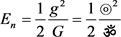
where energy density $E_n=\frac{1}{2}\frac{g^2}{G}$ is for gravitational linear field and proposed is for curvilinear field.

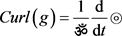
For derivation of gravitational curvilinear field $⊚$ (instead of “h” notation of original text [15] ) in analogy of electromagnetism, let ρ_m is the density of the matter and g (instead of “e” notation of original text [15] ) is the intensity of force or force per unit matter i.e.

$F=g{\rho }_m$,

where the g is the space variation of potential P. Thus

$g=\nabla P$

and potential is found from the distribution of matter as

$P=pot\left({\rho }_m/C\right)={{\displaystyle \sum }}^{\text{}}\frac{{\rho }_m}{4\pi C_r}$,

C = Gravitational constant G⁻¹ and $pot={\nabla }^{-2}$.

Here a matter is allowed to fall together from any configuration to a closer one, the work done by gravitational forcive is expressed by the increase made in

the ${{\displaystyle \sum }}^{\text{}}\frac{1}{2}P{\rho }_m={{\displaystyle \sum }}^{\text{}}\frac{1}{2}\frac{g^2}{G}$ (exhaustion of potential energy) summed through all space.

When a matter ${\rho }_m$ enters any region through its boundary, there is simultaneous convergence of gravitational force into region proportional to ${\rho }_m$. Here if u is the velocity of matter ${\rho }_m$, the ${\rho }_{m}u$ is the density of a current (m/t = flux of matter, kind of potential). It is analogous to a convective current of electrification.

If $C_r={\rho }_{m}u-\frac{g^{.}}{G}$, where $\frac{g^{.}}{G}=\frac{\text{d}g}{G\text{d}t}$

C_r is the circuital flux analogous to Maxwell true current. Being a circuital flux, it is a curl of vector say $⊚$. i.e.

$Curl(⊚)={\rho }_{m}u-\frac{g^{.}}{G}$.

This defines $⊚$ except its divergence, Divergence is arbitrary and may be made zero. Now $⊚$ is analogue to magnetic force, for it bares the same relation to flux of matter as magnetic flux does. We have

$⊚=CurlPot{C}_r$, $A=pot{C}_r$ therefore for instantaneous action

$A=pot\left({\rho }_{m}u\right)$ and

$⊚=Curl\left(A\right)$, $A=m/t$.

Here P is ordinary potential and A = new potential = m/t = flux of P =might be impedance of space-time medium R_G.

Recalling

$Curl(⊚)={\rho }_{m}u-\frac{g^{.}}{G}$, thus

$gCurl(⊚)=g{\rho }_{m}u-g\frac{g^{.}}{G}$.

This is similar to

$Conv{V}_{⊚g}=Fu-U^{.}$,

$Conv\left(V_{⊚g}\right)=\nabla \cdot \left(⊚\times g\right)$

where $U=1/2\left(\frac{g^2}{G}\right)$ but $U^{.}$ is rate of exhaustion potential energy, activity of

force on ${\rho }_m$ is Fu and vector $V_{⊚g}$ defines flux of gravitational energy. This is analogous to flux of electromagnetic energy vector $V_{EH}=E\times H$ found by Oliver himself with poynting.

Interesting outcome by Oliver [15] of above derivation is to acknowledge the field lines of $⊚$ as to follow circular lines perpendicular to mass moving direction axis as magnetic field does around trajectory of charge motion. But directions of flux of energies of electromagnetic system and gravitational system are in reversal mode to each other. This happens due to all matter being alike and attractive while like electrifications repel each other. This ensures very much that the $⊚$ is a gravitational curvilinear field appearing via moving mass.

For radial nature of g, $Curl\left(g\right)$ is resulted into zero. For the finite speed of gravitational force in medium, requirement of $v^2{\nabla }^{2}g=g^{\mathrm{..}}$ suggests undissipated propagation of wave at finite speed. For matter free space ( ${\rho }_{m}u=0$ ), one gets

$-v^{2}Cur{l}^{2}g=g^{\mathrm{..}}$

following

${\nabla }^2=\nabla div-Cur{l}^2.$

But we have

$-Curl(⊚)=\left(\frac{g^{.}}{G}\right)$ and thus

$\frac{v^2}{G}Curlg={⊚}^{.}$, where ${⊚}^{.}=\frac{\text{d}⊚}{\text{d}t}$.

If (instead of “μ” notation of original text [15] ) is a new constant, such that, for $v=c$,

the equation

$\frac{v^2}{G}Curlg={⊚}^{.}$

turns as

or

.

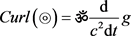
Now moving towards the additional analogies thanks to Oliver [15] as under where $\frac{g^{.}}{1}$, $\frac{E^{.}}{1}$ and $U^{.}$ are time derivatives

(9) Circuital flux → (9) Circuital flux

$Curl(⊚)={\rho }_{m}u-\frac{g^{.}}{G}$ $Curl\left(H\right)={\rho }_{q}u-\frac{E^{.}}{{ϵ}^{-1}}$

(10) Thus $⊚=Curl\left(A\right)$, $A=m/t$ → (10) $H=Curl\left(A\right)$, $A=q/t$.

(11) Flux of gravitational energy is → (11) Flux of Electromagnetic energy is

$Conv{V}_{⊚g}={\left(Fu-U^{.}\right)}_{⊚g}$ $Conv{V}_{EM}={\left(Fu-U^{.}\right)}_{EM}$

(12) → (12) $Curl\left(E\right)=\mu \frac{\text{d}}{\text{d}t}H$

(13) → (13) $ϵ\mu =c^{-2}$

(14) Field lines of $⊚$ is perpen→ (14) Field lines of H is perpendicular

dicular to the axis of moving to the axis of moving

mass. charge.

(15) Flux of gravitated energy → (15) Flux of electromagnetic energy

vector $V_{⊚g}=⊚\times g$ vector $V_{EH}=E\times H$

2.3. Analogy of 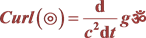to Electromagnetic $Curl\left(H\right)=\frac{d}{c^{2}dt}E/\mu$

One may initiate using Padmanabhan [21] equation 6.132. i.e.

$Curl\left(B_g\right)=\frac{-16\pi G}{c^2}j$,

here j is replaced by

$j=\frac{\text{d}}{\text{d}t}{\displaystyle \int {\rho }_m\text{d}x}$ using $-{\displaystyle \oint j\text{d}f}=\frac{\partial }{\partial t}{\displaystyle \int {\rho }_m\text{d}V}$,

thus

$Curl\left(B_g\right)=\frac{\text{d}}{c^2\text{d}t}{\displaystyle \int -4\pi G{\rho }_m\text{d}x}=\frac{\text{d}}{c^2\text{d}t}{\displaystyle \int \nabla g\text{d}x}$,

the factor 4 is reflection of the fact that is spin—2 field unlike electromagnetic, it is spin—1. Here we adopt spin-1 for gravity wave packet, Finally

One more analogy is

(16) → (16) $Curl\left(H\right)=\frac{\text{d}}{\mu c^2\text{d}t}E$

2.4. Gravitational (Gravitoquagnetic = GEM) Wave Equation in Avail of Quagnetic Field $⊚$

Using the curl equation as

and $B_g=curl{A}_g$,

one gets

$Curl\frac{1}{\text{c}}Curl\left(A\right)=\frac{1}{c^2}\frac{\text{d}}{\text{d}t}g$.

Potential A= vector potential $A_g\times c$, now one gets

$CurlCurl\left(A\right)=-{\nabla }^{2}A+graddiv\left(A\right)=\frac{1}{c}\frac{\text{d}}{\text{d}t}g$

$-{\nabla }^{2}A=\frac{1}{c}\frac{\text{d}}{\text{d}t}g=-\frac{1}{c^2}\frac{{\text{d}}^2}{\text{d}{t}^2}A$.

Therefore

${\nabla }^{2}A-\frac{1}{c^2}\frac{{\text{d}}^2}{\text{d}{t}^2}A=0$

and thus

$\square A=0$,

$\square =\left({\nabla }^2-\frac{1}{c^2}\frac{{\text{d}}^2}{\text{d}{t}^2}\right)$ is D’Alembert operator leads to analogy as

(17) Gravitational (Gravitoquagnetic = GQ) → (17) Electromagnetic = EM

wave equation, $\square A_{GQ}=0$ wave equation, $\square A_{EM}=0$

2.5. Circulation of the Gravitational Vector and Quagnetic Flux

Circulation of the gravitational vector around the contour ( ${\displaystyle \oint g\text{d}l}$ ) is found equal to minus of time derivative the quagnetic flux ( ${\displaystyle \oint ⊚\text{d}f}$ ) through a surface bound by this counter. This is authentication for existence of quagnetic field. Supporting derivation is as

, taking diversion thus

$div⊚=0$ ( $divcurl=0$ ).

Integrating it and applying Gauss’ theorem, it turns as

${\displaystyle \int div⊚\text{d}V}={\displaystyle \oint ⊚\text{d}f}$

and leads to

${\displaystyle \oint ⊚\text{d}f}=0$.

Applying stocks’ theorem for

,

it turns as

${\displaystyle \int Curlg\text{d}f}={\displaystyle \oint g\text{d}l}$.

Therefore

.

Now this circulation of gravitational linear vector ${\displaystyle \oint g\text{d}l}$ ensures existence of curvilinear property of gravitational system which reflects as accumulation of

rate of gravitated curvilinear property $⊚$ as in form of. Analogy with E-M is as under

(18) Circulation of gravitational field is→ (18) Circulation of E-M field is

${\displaystyle \oint E\text{d}l}={\displaystyle \int \frac{\partial H\mu }{\partial t}\text{d}f}$

2.6. Summing Up the Analogies and Justified Extractions

In light of afore said all eighteen analogies and especially considering eighth analogy (as generalized equation of motion for particle in a field), one can conclude here for “Unknown field = curl (A)” relation, the undetected field “Unknown field” is strongly indicating a gravitational curvilinear vector field with complete symmetry with magnetic field H. Equation [21] given below is firmly authenticating existence of curvilinear nature of gravitating system.

$\nabla \times B_g=\frac{-16\pi G}{c^2}j\ne 0$

Here curl of curvilinear induction is survived (not zero). This indicates the completeness [1] of gravitational system. Completeness [1] i.e.

“A vector field can be specified almost completely, if its divergence and curl are given everywhere in space”.

For electromagnetic system formulas, $\nabla \cdot E=4\pi \rho /ϵ$, $\nabla \times E=0$ for stationary electric field and $\nabla \times E=-\partial B/\partial t$ for time varying field are supporting bases of the said completeness [1].

Now one dares to suggest that the parameter-gravitational vector potential [21] $A_{\alpha \left(x\right)}$ of equation given below is existing due to mass current.

$A_{\alpha \left(x\right)}=c{\bar{h}}_{mn}=\frac{4G}{c^2}{{\displaystyle \int }}^{\text{}}\frac{J_{mn}\left(y\right)}{\left|x-y\right|}{\text{d}}^{3}y$

$A_{\alpha \left(x\right)}$ is not merely a perturbation but it is response against change in metric. In simple word, gravitational curvilinear vector potential is responsible to acknowledge counter curvilinear gravitational vector field (New field) to compensate said completeness [1]. In any mass based or charge based system, induced potential due to current is directly in relation with constant say resistance of space-time continuum. Resistances of both the systems are different in formula as well numerical values. Details of medium resistances are cited in present work.

Here quagnetic field $⊚$ is introduced as the name of “Unknown field” (Unknown field = $⊚$ ) of equation “Unknown field = curl (A)”.

Having identical symmetry among charge related system and mass related system, similar mathematical expressions and “completeness [1] ”, similar linear and curvilinear potentials, similar cause (moving particle) for existence for curvilinear quantities, similar emissive properties for linear fields, point to point analogy as well generalized formulation of motion of a particle in a field, analogies by T. Padmanabhan [21], Oliver Heaviside [15] and outcomes of present work rationally demand gravitating curvilinear emissive property means field for as counter reaction against gravitational action.

Probable scenario about above discussion in light of present work is: During such processes like movements of gigantic masses, change in gravity action is responded by reaction of space-time vacuum elasticity in form of quagnetic field. Hence for releasing resulting additional energy due to massive movements to make system stable, not only gravitational but proposed Gravitoquagnetic wave is emitted (like as photon = E-M wave packet). Here by definition weak gravitational waves of finite extend can be explored as wave packet [22]. It may be addressed as Graviton i.e. meaningful sense of Graviton = Gravitoquagnetic wave packet. Importantly such Gravitoquagnetic wave or wave packets, naturally reactive or unreactive towards different types of baryonic substances is matter of study. This scenario is might be similar to reactions of electromagnetic wave and wave packets towards various types of substances of having nature like transparent, opaque, semitransparent, reflector, absorber, refractor, diffractor, homogeneous, inhomogeneous, diffuse, specular, dispersive, non-dispersive etc. properties. And till date it is not known that which substances of nature is how much and why reactive or non-reactive to gravitoquagnetic wave and corresponding wave packet. It might be due to unavailability of man-made gravitoquagnetic wave sources and unavailability of convincing and Omni-acceptable direct detection tools for the same. However recent expensive large-scale instrumental detection of the said gravitational wave should be appreciated respectfully and unanimously without any doubt until solidarity in either optional capacitive suggestion will not be achieved.

3. Gravitoquagnetic Wave

Moreover when the gravitational waves were studied conventionally [23] in curved space-time, averaged pseudo tensor $\langle t^{ik}\rangle$ means $\lambda <t^{ik},L>t^{ik}$ lie between the characteristic distance travelled by wave L with velocity of c and wave length λ. Macroscopically $\langle t^{ik}\rangle$ represent energy density or elasticity. The second order terms of $t^{ik}$ are quadratic in the derivatives of perturbation, $\partial h_{ik}/\partial x^l$ is survived. Those lead to conventional conclusions [23] which are given in inverted coma. “The gravitational wave itself the source of some additional gravitational field”. “Like energy producing it”. Continuing with further conventional conclusion was given as “In such case that the wave itself produces the background field on which it propagates”. Here gravitational wave represents time varying field and hence causes change in gravitational components. Such changes are always opposed by stored energy density of medium via in form of rate of change of natural field and this opponent field is quagnetic field. This was reflected unconsciously in conclusion of aforesaid conventional theory. It is obvious because the general theory of relativity already includes the effect of opponent field or cause while describing gravity. Due to involvement of energy momentum tensor to describe presence of matter and after it is coupled with curvature tensor via Einstein constant, assurance of appearance of coexisting polar field is expected. The energy momentum tensor actually represents energy density of medium at macroscopic level. The energy density of medium as an integrand of action maximally exhibits product of polar or axial fields with their inductions respectively as in the case of electromagnetic action. On the large scale, the time derivative component of $R_{klm}^i$ is in general advocating change in gravitating field and hence inviting opponent field to appear against the change. In light of this, priory having inbuilt polar field properties, the curvature tensor or Ricci tensor or scalar tensor $R\cong G_R$ can be successfully bifurcated into $Q^{lk}{Q}_{lk}$ type dual coexisting polar and axial field tensors for gravity in the present work. All these arguments strongly recommend existence of quagnetic field and hence gravitoquagnetic wave.

4. Estimation of Quagnetic Field $⊚$

In the flat space-time continuum, gravitating effect occurs in presence of mass. The space-time geometry is distorted in proportion to mass. Space-time geometry is not infinitely stretched in the presence of mass. Unknown factor may be elasticity of space-time medium opposes the change in space-time geometry state. Equilibrium between elasticity and presence of mass limits the distortion in space-time medium. Hence not only mass but two factors decide the amount of resultant distortion means gravity. If the space-time geometry is stretched by the action due to mass, the amount of reaction as retainment of geometry by elasticity of medium causes equilibrium. Elasticity of space-time medium decides the amount of energy stored in unit volume. It also decides rate of opposing action per unit volume and hence it is translated as rate of change of natural opponent field. Energy density or elasticity of medium is referred as opposing action against mass effect. Opposing action is in turn translated as the natural opponent field. This natural field naturally opposes the change in state which is often due to presence of mass. Opposing action is rate of change of moment of inertia of the space-time medium. Finally the opponent factor against change in space-time geometry is a counter field to gravitating field and it is related to moment of inertia of space-time medium. The field is defined as rate of change of moment of inertia per volume means opposing action per volume. In other words the field is defined as angular momentum per volume. Symbol and dimensions of the opponent field is $⊚=M/LT$ and unit is Kilogram/(Meter-Second) similar to magnetic field $H=Q/LT$ Coulomb/(Meter-Second).

After the said equilibrium, gravity in proportion of particular mass is set. If any perturbation alters the gravity or any moving object holds inertial acceleration in priory stretched but balanced space-time geometry, the effect of quagnetic field or gravitomagnetic field and obviously related inertia appear. Nature of both i.e. gravimagnetic field and inertia is to oppose the changes due to foreign disturbance accordingly. In short, change in gravity exhibits change in geometry. The change in geometry is invariably opposed by quagnetic field conventionally known as effect of inertia or space-time elasticity.

4.1. Dependency of Curvature Tensor on Presence of Mass and the Space-Time Elasticity as Well Quagnetic Field

Aforesaid discussion gives look like a stationary mass creates gravitomagnetic type field! But the entire scenario is realizing about the event of prompt appearance of stationary mass at flat space-time geometry. The prompt appearance of mass, it may be due to concentration of amount of energy which is compatible to elementary mass at a point or pair production type event. Suppose referring Cartesian coordinates x = xx, y = yy and z = 0 for flat space-time planar fabric, the promptly appeared point mass is vibrating in −z direction in damping manner and localized at z = −g point after equilibrium. Now at this stage, illustration of reaction of space-time geometry against the action of the prompt presence of mass is exercised. In short, right before the said equilibrium, the promptly appeared mass is set in damping vibrating mode under the effect of retainment nature of elasticity of space-time geometry-fabric. For time being such resultant damping vibrational mode of mass explores to and fro movements of mass in negative z direction. These movements invite curvilinear magnetic type of gravitational activity. In this line, the equilibrium is believed to deform flat space-time fabric shape down to z = −g point from z = 0 point of the space-time geometry with two said causes. Such deformation of space-time obviously regards to curved stable-balanced shape of the space-time geometry. This is known as conventional gravity. In real picture, apart from space-time geometry fabric modelling, when the three dimensional spatial flat space is disturbed by the promptly appeared spherical shaped mass, in actual manner the priory homogenous space-time is contracted now intensely in damping vibrating mode in vicinity of spherical mass by keeping the mass stationary. The space-time is gradually becoming lesser intensified as radial distance from center of mass is increased. Here

the components of scalar curvature of space-time are given as ${\Gamma }_{ik}^l=\frac{\partial A^i}{\partial x^k\times A_l}$ while the scalar curvature R is given also as

$R\cong G_R=g^{ik}\left({\Gamma }_{il}^m{\Gamma }_{km}^l-{\Gamma }_{ik}^l{\Gamma }_{lm}^m\right)$.

By analyzing these two formulas, it is obvious that the time derivative component x⁰ of christoffel symbol leads to ${\Gamma }_{00}^{l}c=\frac{\partial A^0}{\partial t\times A_l}$, thus in general it is ${\Gamma }_{00}^{\alpha }=\partial \varnothing \frac{1}{\partial x^{\alpha }{c}^2}$.The term ${\Gamma }_{00}^{l}c=\frac{\partial A^0}{\partial t\times A_l}$ is quite similar to decay constant formula for radioactive decay $\lambda$ i.e. $\lambda =-\frac{\partial N}{\partial t\times N}$ where N is total remaining un-decayed atoms at time t = t seconds. Thus tentatively ${\Gamma }_{00}^{l}c$ term of formula ${\Gamma }_{00}^{l}c=\frac{\partial A^0}{\partial t\times A_l}$ is representing how much gravitated potential activity $\frac{\partial }{\partial t}{A}^0$ is remaining in stock after travelling t = t seconds radially outside from center of spherical gravitated mass. Here instant gravitated potential is $A_l$ at a time t = t seconds. Similarly for the space derivative component $x^{\alpha }$ of christoffel symbol leads to formula ${\Gamma }_{\alpha \alpha }^l=\frac{\partial A^{\alpha }}{\partial x^{\alpha }\times A_l}$. Now this represents how much amount of the radial gravitated potential $\frac{\partial }{\partial x^{\alpha }}{A}^{\propto }$ is remaining after travelling

$x^{\alpha }={\left(x^2+y^2+z^2\right)}^{\frac{1}{2}}$ meters distance radially outside from center of spherical

gravitated mass. In short the said potential $A^{\propto }$ gradually dies down as the test particle is travelling far from the gravity center. The Christoffel symbol looks like generalization of radioactive decay formula. The Christoffel symbol explores quite stationary gravitating scenario and tries to exhibit indexed or diverged nature of gravitated potential as it is evaluated far and far from the gravitated mass. The derivative of the Christoffel symbol is in general leading to dynamic characteristics of the potential, i.e. Poission type equation

$\Delta \varnothing =R_0^0{c}^2=4\pi k\mu =\frac{4\pi kT}{c^2}$.

Its solution is $\varnothing =-k{{\displaystyle \int }}^{\text{}}\frac{\mu \text{d}V}{r}=-km/r$ conveys gravitational force field via known potential field due to mass density distribution. Concluding afore said para as: $R_0^0=km\Delta \left(1/r\right)/c^2$ certainty indicates $R_0^0\propto$ mass density as well indicates $R_0^0=4\frac{\pi k\mu }{c^2}=\frac{4\pi kT}{c^4}$. It perfectly announces $R_0^0\propto T=\mu c^2$ = energy

density = elasticity of medium. The assumption $T=\mu c^2$ = energy density = elasticity of medium is based on common natural sense i.e. if two identical masses hold same shape and volume dimensions but different elasticities of each, the curvatures of space-time created by both the masses would not be different. Thus it is better to assume $T=\mu c^2$ is as space-time elasticity in place of gravitated mass-matter elasticity. Thus

$R_0^0=\left(\$\right)m\Delta \left(1/r\right)\mu c^2$

leads the compensative term ($) as $\left(\$\right)=\left(4\pi /{⊚}^2\right)$ where $⊚$ is quagnetic field and its dimension is M/LT means Kilogram/(Meter-Second). Thus proportionalities of space-time curvature are obeying two natural causes as per present article argument and causes are mass and elasticity. Here proportionality variable is $\left(4\pi /{⊚}^2\right)$. Here ($) is defined as

Here and dimensional equality $k\mu =g/l$ formulas are used at least to justify role of quagnetic field $⊚$. Thus

$R_0^0\cong \left(4\pi /{⊚}^2\right)m\Delta \left(1/r\right)\mu c^2$

where $⊚$ is curvilinear vector field roles in parallel manner amongst formation of space-time curvature. The curvature is also concerning mass density of gravitated mass and space-time elasticity. On accumulation of the things at large scale the relation of curvature and relevant properties is

$\begin{array}{c}\text{Curvature}\left(R\right)\cong \frac{\text{Mass density}\left(\mu \right)\times \text{Medium Elasticity}\left(\mu c^2\right)}{\text{Square of Quagnetic field}\left({⊚}^2\right)}\\ =\frac{\text{Square of mass current density}\left(J^2\right)}{\text{Square of Quagnetic field}(\; ⊚\; 2\; )}\end{array}$

4.1.1. Estimation of Electromagnetic Curvature (R_EM)

The derivative of invariance electromagnetic field strength is given as

$\frac{\partial }{\partial x^i}{F}_{ik}=\frac{\partial }{\partial x^i}\left\{{\partial }_i{A}_k-{\partial }_k{A}_i\right\}=4\pi \frac{j_i}{cϵ}$.

The electromagnetic curvature (R_EM) can be estimated as

$\begin{array}{c}\text{Curvature}\left(R_{EM}\right)\cong \frac{q\partial }{m{c}^2\partial x^i}{F}_{ik}=\frac{q}{m{c}^2}\frac{\partial }{\partial x^i}\left\{{\partial }_i{A}_k-{\partial }_k{A}_i\right\}\\ =4\pi \frac{q}{m{c}^2}\frac{j_i}{cϵ}=4\pi \frac{q}{m{c}^2}\frac{j_i\times j_i}{cϵ\times j_i}=4\pi \frac{j_i\times j_i}{H^2}\end{array}$

thus electromagnetic curvature is given as

$\text{Curvature}\left(R_{EM}\right)\cong 4\pi \frac{j_i\times j_i}{H^2}\cong \frac{\text{Square of current density}\left(J^2\right)}{\text{square of magnetic field}\left(H^2\right)}$.

Recalling the Curvature (R) for comparison with Curvature (R_EM)

$\text{Curvature}\left(R\right)\cong \frac{\text{Square of mass current density}\left(J^2\right)}{\text{Square of Quagnetic field}\left({⊚}^2\right)}$.

Similarity of dependences of Curvature (R_EM) and Curvature (R) are quite identical for electromagnetic and gravitoquagnetic systems.

Here dimensions of $\frac{q}{m{c}^2}\frac{1}{cϵ\times j_i}$ is obviously similar to inverse of square of magnetic field (H⁻²).

4.1.2. Estimation of the Gravitated Curvature Tensor (R) Analogous to (R_EM)

The gravitated curvature tensor (R) can be defined as below, if and only if the existence of curvilinear quagnetic field $⊚$ is accepted. At this stage, this allows us to assume that to find the equations of motion; the field is given and varied the trajectory of particle. Thus by varying the action one finds

$\delta S=-{{\displaystyle \int }}^{\text{}}\frac{1}{c}\left\{\frac{1}{c}{j}_m^i\delta A_i+\frac{1}{8\pi }{Q}^{ik}\delta Q_{ik}\right\}\text{d}\Omega =0$

where $Q_{ik}=\left\{{\partial }_i{A}_k-{\partial }_k{A}_i\right\}$ and $j_m^i$ is mass current density. After some simplification one gets

${{\displaystyle \int }}^{\text{}}\left\{\frac{1}{c}{j}_m^i+\frac{1}{4\pi }\frac{\partial }{\partial x^k}{Q}^{ik}\right\}\delta A_i\text{d}\Omega =0$.

Taking coefficients of $\delta A_i$ is zero; the derivative of gravitoquagnetic field tensor $\frac{\partial }{\partial x^k}{Q}^{ik}$ is resulted in to mass current density as

$\frac{\partial }{\partial x^k}{Q}^{ik}=\frac{\partial }{\partial x^i}\left\{{\partial }_i{A}_k-{\partial }_k{A}_i\right\}=4\pi \frac{j_m^i}{c}G$.

Once this sets, for together the two succeeding equations i.e. i = 2, 3, the term

$Curl(⊚)-\frac{\partial g}{c\partial t}=4\pi \frac{j_m^i}{c}G$ also exists and

for i = 0,

$div\left(g\right)=4\pi \rho$.

Thus Gravitated second pair of Maxwellian type equation can be obtained. Thus

$R_{ambn}\cong \frac{\partial }{\partial x^i}\left\{{\partial }_i{A}_k-{\partial }_k{A}_i\right\}/A_l=\left(Curl(⊚)-\frac{\partial g}{c\partial t}\right)/A_l$.

Moreover it also guarantees to have zero space-time curvature in absence of mass i.e. $4\pi \frac{j_m^i}{c}G=0$ and at that same time $Curl(⊚)=\frac{\partial g}{c\partial t}$. Means in absence

of mass, rate of change in gravity is capable to produce curly quagnetic field $⊚$. This clearly suggests that the curvature of space-time is consisting of two gravitated fields linear g and curvilinear $⊚$ components.

It is analogous to electromagnetic system formula as

$\frac{\partial }{\partial x^i}{F}_{ik}=\frac{\partial }{\partial x^i}\left\{{\partial }_i{A}_k-{\partial }_k{A}_i\right\}=4\pi \frac{j_m^i}{cϵ}=\left(Curl\left(H\right)-\frac{\partial E}{c\partial t}\right)$

Here potentials A_k and A_i are adopted either electromagnetic or gravitated systems as per requirements of argument.

Now switch over to gravitated curvature form, it is given as

$R_{ambn}\cong g_{al}\left({\partial }_b{\Gamma }_{mn}^l-{\partial }_n{\Gamma }_{mb}^l\right)=\frac{\partial }{\partial x^b{A}_l}\left\{\frac{\partial A_m}{\partial x^n}-\frac{\partial A_n}{\partial x^m}\right\}$.

Analyzing only $R_{ambn}\cong {\partial }_b{\Gamma }_{mn}^l$ for wide purpose as to have dependences of curvature, thus

$R_{ambn}\cong {\partial }_b{\Gamma }_{mn}^l=\frac{\partial }{\partial x^i}{\Gamma }_{ij}^l=\frac{2}{c^2}\frac{\partial }{\partial x^i}\left\{\frac{\partial A_i}{\partial x^j}-\frac{\partial A_j}{\partial x^i}\right\}$.

It leads to

$\frac{\partial }{\partial x^i}{\Gamma }_{ij}^l=\frac{2}{c^2}\frac{\partial }{\partial x^k}{Q}^{ik}=8\pi \frac{j_m^i}{c^3}G$.

Here similar type gravitated formulation using $\Gamma$ [11] is given as using and dimensionally. Thus approximately

. Thus

.

Here $j_m^i$ is mass current density.

Concluding Sections 4.1, 4.1.1 and 4.1.2, the curvature (R) can be declared as a dependent term of mass density and energy density of space-time continuum. It also cares about mass current density and adjoined the quagnetic field for gravitated system and similarly it also cares about current density as well adjoined magnetic field for electromagnetic system.

4.2. Dependency of Product of Curvature Tensor on Presence of Mass and the Space-Time Elasticity as Well Mass Current

In connection of Section 2.1 of present article, the product of equations $R_0^0{R}_0^0$ is given using

$R_0^0=\frac{4\pi kT}{c^4}$ and $R_0^0=km\Delta \left(1/r\right)/c^2$

as

$\begin{array}{c}{R}_0^0{R}_0^0=\left(4\pi kT/c^4\right)\left(km\Delta \left(1/r\right)/c^2\right)\\ =\left(4\pi k/c^4\right)\left(k/c^2\right)m\Delta \left(1/r\right)\mu c^2\\ =(\#)m\Delta \left(1/r\right)\mu c^2\end{array}$

Here the compensative term (#) is given as

.

where mass current is $I_m$, and formulas are used. And dimensionally $B_{g}l=c$ is adopted at least to explore the role of mass current. Thus

$R_0^0{R}_0^0\cong \left(16{\pi }^3/I_m^2\right)\left(m\Delta \left(1/r\right)\mu c^2\right)$.

Here used but still unknown new formulas are derived and explained in this article Quagnetic field part (I) and accepted article Quagnetic field part (II) in JHEPGC [18]. In general, product of curvatures RR is also dependent on two said causes the mass and the space-time elasticity but here the key property is mass current. i.e.

$\text{Curvature}\left(RR\right)=\left(16{\pi }^3/{\text{mass current}}^2\right)m\Delta \left(1/r\right)\mu c^2$.

Analyzing identical dependencies upon the mass effect and the space-time elasticity effect of curvature tensor R and their product RR, respectively the quagnetic field $⊚$ and the mass current $I_m$ are found as key properties.

If the derivative of mass current exists i.e. $\frac{\partial I_m}{\partial x^i}\ne 0$, $i=1,2,3$, the quagnetic field $⊚$ appears and being a cause of existence of

$R_0^0\cong \left(4\pi /{⊚}^2\right)m\Delta \left(1/r\right)\mu c^2$.

If the mass current is constant with respect to translational motions, it survives the curvature product concerning mass current as

$R_0^0{R}_0^0\cong \left(16{\pi }^3/I_m^2\right)\left(m\Delta \left(1/r\right)\mu c^2\right)$.

On accumulation of the things at large scale, the relation for curvature RR and relevant properties is

$\begin{array}{c}\text{Curvature}\left(RR\right)\cong \frac{\text{Mass density}\left(\mu \right)\times \text{Medium Elasticity}\left(\mu c^2\right)}{\text{Square of mass current}\left(I_m^2\right)}\\ =\frac{\text{Square of mass current density}\left(J^2\right)}{\text{Square of mass current}\left(I_m^2\right)}\end{array}$

4.2.1. Estimation of Electromagnetic Curvature (RR_(EM))

The derivative of invariance electromagnetic field strength is

$\frac{\partial }{\partial x^i}{F}_{ik}=\frac{\partial }{\partial x^i}\left\{{\partial }_i{A}_k-{\partial }_k{A}_i\right\}=4\pi \frac{j_i}{cϵ}$.

The electromagnetic curvature (R_EM) can be estimated as

$\text{Curvature}\left(R_{EM}\right)\cong \frac{q\partial }{m{c}^2\partial x^i}{F}_{ik}=\frac{q}{m{c}^2}\frac{\partial }{\partial x^i}\left\{{\partial }_i{A}_k-{\partial }_k{A}_i\right\}=4\pi \frac{q}{m{c}^2}\frac{j_i}{cϵ}$.

Thus electromagnetic curvature (RR_(EM)) is given by simple product of $\frac{\partial }{\partial x^i}{F}_{ik}\times \frac{\partial }{\partial x^i}{F}^{ik}$ as

$\begin{array}{c}\text{Curvature}\left(R{R}_{\left(EM\right)}\right)\cong \frac{q\partial }{m{c}^2\partial x^i}{F}_{ik}\frac{q\partial }{m{c}^2\partial x^i}{F}^{ik}\\ =4\pi \frac{q}{m{c}^2}\frac{j_i}{cϵ}\times 4\pi \frac{q}{m{c}^2}\frac{j_i}{cϵ}=16\frac{{\pi }^2{j}_i^2}{I_q^2}\end{array}$

Here dimensions of ${\left(\frac{q}{m{c}^2}\frac{1}{cϵ}\right)}^2$ is obviously matching within verse of square of current $I_q^{-2}$. Hence

$\text{Curvature}\left(R{R}_{\left(EM\right)}\right)\cong \frac{\text{Square of current density}\left(j_i^2\right)}{\text{square of current}\left(I_q^2\right)}$

4.2.2. Estimation of the Gravitated Curvature Tensor (RR) Analogous to (RR_(EM))

Recalling formula of Section 2.1.2, thus gravitoquagnetic system formula is given as

$\frac{\partial }{\partial x^k}{Q}^{ik}=\frac{\partial }{\partial x^i}\left\{{\partial }_i{A}_k-{\partial }_k{A}_i\right\}=4\pi \frac{j_m^i}{c}G$.

It is analogous to electromagnetic system formula given as

$\frac{\partial }{\partial x^i}{F}_{ik}=\frac{\partial }{\partial x^i}\left\{{\partial }_i{A}_k-{\partial }_k{A}_i\right\}=4\pi \frac{j_i}{cϵ}$.

Here potentials A_k and A_i are adopted either electromagnetic or gravitated systems as per requirements. Now switch over to gravitated curvature form, it is given as

$R_{ambn}\cong g_{al}\left({\partial }_b{\Gamma }_{mn}^l-{\partial }_n{\Gamma }_{mb}^l\right)=\frac{\partial }{\partial x^b{A}_l}\left\{\frac{\partial A_m}{\partial x^n}-\frac{\partial A_n}{\partial x^m}\right\}$.

Analyzing only $R_{ambn}\cong {\partial }_b{\Gamma }_{mn}^l$, one gets

$R_{ambn}\cong {\partial }_b{\Gamma }_{mn}^l=\frac{\partial }{\partial x^i}{\Gamma }_{ij}^l=\frac{2}{c^2}\frac{\partial }{\partial x^i}\left\{\frac{\partial A_i}{\partial x^j}-\frac{\partial A_j}{\partial x^i}\right\}$.

It leads to

$\frac{\partial }{\partial x^i}{\Gamma }_{ij}^l=\frac{2}{c^2}\frac{\partial }{\partial x^k}{Q}^{ik}=8\pi \frac{j_m^i}{c^3}G$.

Here similar type gravitated formulation using $\Gamma$ [11] is given as using and dimensionally. Thus approximately

.

where $j_m^i$ is mass current density. Thus Curvature (RR) is estimated as

$\text{Curvature}\left(RR\right)\cong \left(R_{ambn}\right){\left(R_{ambn}\right)}^{*}\cong \frac{2}{c^2}\frac{\partial }{\partial x^i}\left\{\frac{\partial A_i}{\partial x^j}-\frac{\partial A_j}{\partial x^i}\right\}\times \frac{2}{c^2}\frac{\partial }{\partial x^i}\left\{\frac{\partial A^i}{\partial x^j}-\frac{\partial A^j}{\partial x^i}\right\}$.

Therefore

$\begin{array}{c}\text{Curvature}\left(RR\right)={\left(8\pi \frac{j_m^i}{c^3}G\right)}^2=64{\pi }^2\frac{{\left(j_m^i\right)}^2}{I_m^2}\\ \cong \frac{\text{Square of mass current density}\left(j_m^2\right)}{\text{Square of mass current}\left(I_m^2\right)}\end{array}$

Here $\frac{G^2}{c^6}$ is obviously dimensionally match the term $I_m^{-2}$.

Concluding Sections 4.2, 4.2.1 and 4.2.2, the curvature (RR) can be declared as it depends on mass density and energy density of space-time continuum. It also cares about mass current density and the mass current for gravitated system and similarly it also cares about current density as well current for electromagnetic system. In support of this statement it is already mentioned [21] using Einstein equations that the measured scalar curvature is equivalent to 16 πk times of the measured energy density.

Roughly illustrating that the space-time curvature R is also dying down as radial distance from center of the mass is increased. Macroscopically $R=\left(\frac{4\pi k}{c^4}\right)T$ and

$T=\mu c^2$, where $\mu$ is medium density. So as curvature R decreases with decrement of weightage of $\Gamma$, it also leads to decrement of medium density μ with decrement of elasticity of medium as well. Tentative to and fro motion of mass makes this situation dynamic and obvious trend to achieve the equilibrium causes the motion damped. This explores indexed intensity decrement of space-time density around the presence of the spherical gravitated mass. Relatively, such indexed decreasing manner type density of vibrating space-time in vicinity of literally stationary promptly appeared mass illusionary makes the mass to be appeared as in vibrating mode.

4.3. Argument of the Present Article and Literature Support

Argument of the present article is: The general theory of relativity initiated its analyzing formulation of gravity after the said equilibrium. Thus the space-time Riemannian curvature tensor $R_{\mu \nu \rho \sigma }$ existing in presence of mass-energy is actually resultant state of said equilibrium. Obviously the Riemannian tensor R individually and product of Riemannian tensors RR are consisting effects of the said both the components say, mass effect and elasticity effect. Thus aim of the present article is pin pointedly collimated to extract gravitational component as well quagnetic or gravitomagnetic component from curvature terms R as well from their product RR. Detailed proceeding is given as under.

The gauge invariance of electromagnetism under electromagnetic potential gauge formula [24] $A_{\mu }\to A_{\mu }+{\partial }_{\mu }\lambda$ is obtained. Here invariance of electromagnetic field strength is given as i.e. $F_{ik}={\partial }_i{A}_k-{\partial }_k{A}_i$. The similar mathematical exercise is done for $F_{ik}$ type gravitational issue. Where the gravitational gauge transformation of perturbation [24] is given as $h_{\mu \nu }^{\left(ϵ\right)}=h_{\mu \nu }+2ϵ{\partial }_{\left(\mu \xi \nu \right)}$. It leaves the space-time curvature unchanged or $\delta R_{\mu \nu \rho \sigma }=0$. The electromagnetic scalar field tensor $F_{ik}{F}^{ik}=8\pi \left(H^2\mu -E^2ϵ\right)$ is found invariant. Similarly gravitated Riemannian space-time curvature tensor

$R^{\ast }\cdot R\equiv R^{\ast \left(\mu \nu \rho \sigma \right)}{R}_{\mu \nu \rho \sigma },R^{\mu \nu \rho \sigma }={\epsilon }^{\mu \nu \alpha \beta }\frac{1}{2}{R}_{\alpha \beta }^{\rho \sigma }{R}^{\mu \nu \rho \sigma }$

is found invariant [11]. Here $R^{\ast \left(\mu \nu \rho \sigma \right)}$ is dual to $R_{\mu \nu \rho \sigma }$. For example, for the gravitated system having angular momentum J and the rotating mass M. Thus it obviously holds the volume density of angular momentum J. The J/(volume) indicates dimensions of quagnetic field $⊚$. In that line, the invariant $R^{\ast }\cdot R$ have angular momentum J holding non-zero value for Kerr metric. Kerr metric is generated by angular momentum J and mass M. Slight differently having angular momentum J is with zero value for Schwarzschild metric. It is generated by mass M only. Thus space-time curvature, generated by angular momentum is manifestly displayed by the said curvature invariant $R^{\ast }\cdot R$. For example a point mass metric generated by earth and sun, where finding is $R^{\ast }\cdot R\cong G\cdot H$. H is magnetic type gravitational field [11], i.e. $H=⊚$ named quagnetic field. For a

test particle moving with speed of v, the H is formulated as $H\cong \frac{v\times g}{G}\cong ⊚$. In

parallel, in the standard parameterized post Newtonian (PPN) framework [5] for an isolated, weakly gravitating and slowly rotating body, the PPN space-time metric coefficients involving its angular momentum represent the off diagonal terms. The off diagonal terms are presented as

$g_{0i}=\frac{\gamma +1}{c^2}{\nu }_i$, $i=1,2,3$.

Here the potential $\nu =\frac{GS}{c{r}^3}\times r$, S is the momentum and $\gamma =1$ for General theory of relativity. Whenever term s/r³ is appeared in any key formula, it translates that the quagnetic field $⊚=s/r^3$ is invariably included and whereas $\frac{S}{r^3}\times r$ indicates inclusion of presence of mass current. The potential term is

adopted from formula of the gravitomagnetic B_g field effect, where B_g is predicted for test body far from the localized rotating body with angular momentum = S. The gravitomagnetic field B_g effective to test body can be written as

$B_g=\frac{G}{c^2}\frac{1}{r^3}\left[S-3\left(S\cdot r_0\right)r_0\right]$.

This B_g field affects the test particle moving with velocity v with a non-central acceleration as

$A_{GM}=-2\frac{v}{c}\times B_g$.

Thus

$A_{GM}=-2\frac{v}{c}\frac{G}{c^2}\frac{1}{r^3}\left[S-3\left(S\cdot r_0\right)r_0\right]$.

Where S is the angular momentum of the source, r is the distance between the source and test particle, r₀ is the unit vector. Naturally effect of B_g on test particle at distance r is A_GM. This A_GM effect on test particle is the main cause of Lense-Thirring effect, gyroscope precession and Gravitomagnetic Clock effect.

Now back to PPN method where the resulting Christoffel symbols [11] including angular momentum S via potential ${\nu }_i,i=1,2,3$ entering the geodesic equation of motion as

${\Gamma }_{0j}^i=-\frac{\gamma +1}{c^2}\left(\frac{\partial }{\partial x^j}{\nu }_i-\frac{\partial }{\partial x^i}{\nu }_j\right)$.

The expression $\left(\frac{\partial }{\partial x^j}{\nu }_i-\frac{\partial }{\partial x^i}{\nu }_j\right)$ represents g-field and its gravitated scalar

$Q^{ik}{Q}_{ik}$ exhibit square of g-field. Square of g-field $\propto$ energy density and potential ${\nu }_i$ with having angular momentum component is part of metric off diagonal terms which are directly related to gravitomagnetic or quagnetic field. Moreover, it is to say [21] that gauge transformation leaves the curvature tensor $R_{mnr}^s$ invariant. So,

$R_{ambn}\cong g_{al}\left({\partial }_b{\Gamma }_{mn}^l-{\partial }_n{\Gamma }_{mb}^l\right)=\frac{\partial }{\partial x^b{A}_l}\left\{\frac{\partial A_m}{\partial x^n}-\frac{\partial A_n}{\partial x^m}\right\}$

is invariant. This term $R_{mnr}^s$ holds invariance nature individually. In the line of this, in the present article, both the causes of gravity i.e. gravitational field as well quagnetic field are extracted from the conventional-traditional action function of gravitated system. The action function is constructed by general theory of relativity using Riemannian space-time curvature tensor.

The Riemannian tensor is invariant and without any doubt carrying two causes of resultant gravity, those are, firstly field due to mass effect i.e.—gravitational field and secondly field due to elasticity of space-time i.e. —quagnetic field or gravitomagnetic field. The PPN approximation is solid backbone to present article argument via providing the resultant Christoffel symbols of geodesic equation motion. The resultant Christoffel symbols are appeared having formulation similar

to electromagnetic field tensor i.e. expression $\left(\frac{\partial }{\partial x^j}{\nu }_i-\frac{\partial }{\partial x^i}{\nu }_j\right)$. The expression related to linear and curvilinear fields is common in both the electromagnetic

and gravitoquagnetic or gravitoelectromagnetic systems. Rough estimation indicates us like: The Riemannian expression is constructed with square of Christoffel symbols and derivative of Christoffel symbols. It gives look similar as product of electromagnetic field tensor with its dual to explore scalar property. This is again tempting to predict that not only the product of Riemannian curvature tensor with its dual tensor but merely single individual Riemannian tensor can also represent the curvature of space-time fabric. Single individual Riemannian tensor is sufficiently capable to exhibit gravitational as well quagnetic or gravitomagnetic field components in form of energy density. Because fundamentally the curvature is a resultant state of the said two causes. Apart from philosophical argument based presentation of existence of the said two fields, mathematically it is proved here that product

$R^{\ast }\cdot R\equiv R^{\ast \left(\mu \nu \rho \sigma \right)}{R}_{\mu \nu \rho \sigma },R^{\mu \nu \rho \sigma }={\epsilon }^{\mu \nu \alpha \beta }\frac{1}{2}{R}_{\alpha \beta }^{\rho \sigma }$

as well as single Riemannian scalar $R\cong G_R$ of gravitated action function is firmly presenting existence of both the said fields because single Riemannian scalar $R\cong G_R$ holds both the said fields as its primitive components. This is really a full throttle mathematical support to present article arguments.

4.4. Gravitating Field Tensors

The electromagnetic action [25] $S_f$ is given as part of actions which depends only on field itself. The electromagnetic tensors are $F_{ik}$ and $F^{ik}$ and to meet scalar action, their product is chosen as scalar. The $S_f$ is given as

$S_f=\left(\frac{1}{16\pi c}\right){\displaystyle \int F_{ik}{F}^{ik}\text{d}\Omega }$, where $\text{d}\Omega =c\text{d}t\text{d}x\text{d}y\text{d}z$

Similar to the electromagnetic action integrand

$F_{ik}{F}^{ik}=8\pi \left(H^2\mu -E^2ϵ\right)$ form,

the gravitoquagnetic action integrand as

is not available. It is because of unavailability of gravitating curvilinear vector field. Where is inverse of gravitating permeability related to Einstein constant [19]

$\chi =\frac{8\pi k}{c^2}$ as. The same is discussed at end of topic. Thus the variation

of action S_g for gravitating system [20] is given differently compared to electromagnetic system in the form of Riemannian tensors as under.

$\delta S_g=\left(-\frac{C^3}{16\pi k}\right)\delta {\displaystyle \int G_R\sqrt{-g}\text{d}\Omega }$, $\text{d}\Omega =c\text{d}t\text{d}x\text{d}y\text{d}z$.

Here k =G is universal gravitational constant. $G_R\sqrt{-g}\cong R\sqrt{-g}$ is scalar curvatures or scalar integrands. i.e. $\delta {\displaystyle \int R\sqrt{-g}\text{d}\Omega }=\delta {\displaystyle \int G_R\sqrt{-g}\text{d}\Omega }$ + vanished an integral during variation over a hyper surface surrounding the four-volume.

Where $R=g^{ik}{R}_{ik}=g^{il}{g}^{km}{R}_{iklm}$ where $R_{ik}$ is Ricci tensor and $R_{iklm}$ is curvature tensor or Riemann tensor. The scalar $G_R\cong R$ is given as

$G_R\cong R=–g^{ik}\left({\Gamma }_{il}^m{\Gamma }_{km}^l-{\Gamma }_{ik}^l{\Gamma }_{lm}^m\right)$,

$\Gamma$ is Christoffel symbol, given as ${\Gamma }_{ik}^l=\partial A^i/\left(\partial x^k{A}_l\right)$. Therefore

$G_R=-g^{ik}\left(\frac{{\Gamma }_{im}^m}{A_l}\right)\left\{\frac{\partial A_k}{\partial x^l}-\frac{\partial A_l}{\partial X^k}\right\}$,

Here

$\left\{\frac{\partial A_k}{\partial x^l}-\frac{\partial A_l}{\partial X^k}\right\}=Q_{lk}\sqrt{G}$

is gravitating field tensor like electromagnetic field tensor $F_{ik}$, where A_k and A_l are gravitational potentials. Therefore the tensor G_R is given as

$G_R=-g^{ik}\left(\frac{{\Gamma }_{im}^m}{A_l}\right)\left\{Q_{lk}\right\}\sqrt{G}$.

The existence of expression like $Q_{lk}$ for gravitating system, ensuring to hope about coexisting curvilinear vector field in contravariant version also. Hence $Q_{lk}=\left(g,\text{newfield}\right)$ and $Q^{lk}=\left(-g,\text{newfield}\right)$ are expected. If $⊚$ symbol is adopted for that new curvilinear vector field, thus $Q_{lk}=\left(g,⊚\right)$ and $Q^{lk}=\left(-g,⊚\right)$ are symbolized accordingly. Similar to the electromagnetic field tensor, $Q^{lk}$ and $Q_{lk}$ both hold polar and axial potential like $A_l=\left(\varphi ,-A\right)$ and $A^l=\left(\varphi ,A\right)$ respectively.

Where $Q_{lk}$ is given as

$Q_{lk}=\left(\begin{array}{cccc}0& g_x& g_x& g_x\\ -g_x& 0& -{⊚}_z& {⊚}_y\\ -g_x& {⊚}_z& 0& -{⊚}_x\\ -g_x& -{⊚}_y& {⊚}_x& 0\end{array}\right)$

and, $Q^{lk}$ is given as

$Q^{lk}=\left(\begin{array}{cccc}0& -g_x& -g_x& -g_x\\ g_x& 0& -{⊚}_z& {⊚}_y\\ g_x& {⊚}_z& 0& -{⊚}_x\\ g_x& -{⊚}_y& {⊚}_x& 0\end{array}\right)$

Both are representing two fields “g” and “ $⊚$ ” = $\frac{M}{LT}$.

4.5. Estimation of Two Gravitating Fields Comparing Symmetries of Electromagnetic and Gravitoquagnetic Action Functions

Using generalized Stock theorem the integral over a four dimensional closed curve is transformed in to an integral over the surface as under.

${\displaystyle \oint A_i\text{d}{x}^i}={\displaystyle \int \text{d}{f}^{ki}\partial A_i/\partial x^k}=\frac{1}{2}{\displaystyle \int \text{d}{f}^{ik}\left\{\frac{\partial A_k}{\partial x^i}-\frac{\partial A_i}{\partial x^k}\right\}}$,

$\partial A_i/\partial x^k=\frac{1}{2}\left\{\frac{\partial A_k}{\partial x^i}-\frac{\partial A_i}{\partial x^k}\right\}$.

And inspiring from PPN approximation [11], the Christoffel symbols are given as

${\Gamma }_{0j}^i=-\frac{\gamma +1}{c^2}\left(\frac{\partial }{\partial x^j}{\nu }_i-\frac{\partial }{\partial x^i}{\nu }_j\right)$.

Therefore

$\begin{array}{c}{G}_R=-g^{ik}/\left(2A_m{A}_l\right)\left\{\frac{\partial A_m}{\partial x^i}-\frac{\partial A_i}{\partial X^m}\right\}\left\{\frac{\partial A_k}{\partial x^i}-\frac{\partial A_l}{\partial X^k}\right\}\\ =\left(\frac{-g^{ik}}{2A_m{A}_l}\right)Q_{im}{Q}_{lk}G=\frac{\left(-g^{ik}/g^{li}{g}^{km}\right)Q^{lk}{Q}_{lk}G}{2A_m{A}_l}\end{array}$

Hence

$G_R=-g^{ik}\left(\frac{{\Gamma }_{im}^m}{A_l}\right)\left\{\frac{\partial A_k}{\partial x^l}-\frac{\partial A_l}{\partial X^k}\right\}=\frac{\left(-g^{ik}/g^{li}{g}^{km}\right)Q^{lk}{Q}_{lk}G}{2A_m{A}_l}$.

Dimension of $Q^{lk}{Q}_{lk}$ is equal to energy density. i.e.

The gravitated invariant field tensor $\left\{Q^{lk}{Q}_{lk}\right\}$ like electromagnetic $F_{ik}{F}^{ik}$ can be obtained using product of gravitational curvature tensor as

$G_{R\left(Q_{lk}\right)}=-g^{ik}\left(\frac{{\Gamma }_{im}^m}{A_l}\right)\left\{\frac{\partial A_k}{\partial x^l}-\frac{\partial A_l}{\partial X^k}\right\}=-g^{ik}\left(\frac{{\Gamma }_{im}^m}{A_l}\right)Q_{lk}\sqrt{G}$,

$\begin{array}{c}{G}_{R\left(Q^{lk}\right)}=-g^{ik}\left(\frac{{\Gamma }_{ik}^l}{A_m}\right)\left\{\frac{\partial A_m}{\partial x^i}-\frac{\partial A_i}{\partial X^m}\right\}=-g^{ik}\left(\frac{{\Gamma }_{ik}^l}{A_m}\right)Q_{im}\sqrt{G}\\ =-g^{ik}\left(\frac{{\Gamma }_{ik}^l}{A_m}\right)Q^{lk}\sqrt{G}/g^{li}{g}^{km}\end{array}$

thus

$\begin{array}{c}{G}_{R\left(Q_{lk}\right)}{G}_{R\left(Q^{lk}\right)}=-g^{ik}\left(\frac{{\Gamma }_{im}^m}{A_l}\right)Q_{lk}\sqrt{G}\left(-g^{ik}\left(\frac{{\Gamma }_{ik}^l}{A_m}\right)Q^{lk}\sqrt{G}\right)\\ =G{g}^{ik}{g}^{ik}\left(\frac{{\Gamma }_{im}^m}{A_l}\frac{{\Gamma }_{ik}^l}{A_m}\right)\left\{Q^{lk}{Q}_{lk}\right\}\end{array}$

Here the product of Riemannian invariant space-time curvature tensor like $G_{R\left(Q_{lk}\right)}{G}_{R\left(Q^{lk}\right)}$ directly resulted as the gravitated invariant field tensor $\left\{Q^{lk}{Q}_{lk}\right\}$ similar to electromagnetic invariant field tensor $F_{ik}{F}^{ik}=8\pi \left(H^2\mu -E^2ϵ\right)$ but

additional $\left(\frac{{\Gamma }_{im}^m}{A_l}\frac{{\Gamma }_{ik}^l}{A_m}\right)$ term of the product $G_{R\left(Q_{lk}\right)}{G}_{R\left(Q^{lk}\right)}$ seems like one more gravitational term as square of gravitating field is appeared. Importantly here we are examining the case on generalized manner by having derivatives respect to both $x^0$ and $x^{\alpha }$, not giving space to specialize only $x^0$ component to rationalize the additional $\left(\frac{{\Gamma }_{im}^m}{A_l}\frac{{\Gamma }_{ik}^l}{A_m}\right)$ terms in required scalar forms. At least for this case, instead of considering $G_{R\left(Q_{lk}\right)}{G}_{R\left(Q^{lk}\right)}$ the whole treatment puts itself into

compulsion to consider the single Riemannian tensor term. Here a single curvature tensor likes $R_{\mu \nu \rho \sigma }$ or Ricci $R_{\mu \nu }$ or Riemannian scalar R is not seen in relevant literature as to exhibit the sum of energy densities of both the gravitational and gravitomagnetic or quagnetic components. However in the present formulation in favor of present article argument (curvature is resultant state of equilibrium of mass effect and elasticity effect), a single curvature tensor G_R of gravitated action function individually sufficient to explore the sum of energy densities of both the gravitational and gravitomagnetic or quagnetic components. Why and how is concluded in brief, i.e. curvature of space-time is shaped due to gravity. Gravity is believed to appear in accord to mass-energy. But at intermediate stage of equilibrium between believed gravity due to mass-energy effect and the space-time fabric elasticity, the elasticity plays opposing role against the mass effect to truncate infinite stretching. Thus resultant curvature is appeared as consistence of two said causes. Obviously formulation of such curvature exhibits both the physical and mathematical characteristics of its primitive components. i.e. complete existence of the curvature is due to gravity as well quagnetic or gravimagnetic activities.

The curvature and action integral are given using only single curvature term, those are given as

$G_R=\frac{\left(-g^{ik}/g^{li}{g}^{km}\right)Q^{lk}{Q}_{lk}G}{2A_m{A}_l}$,

$S_g=-\left(C^3/16\pi k\right){\displaystyle \int G_R\sqrt{-g}\text{d}\Omega }=-\left(C^4/16\pi c\right){\displaystyle \int \frac{-g^{ik}/g^{li}{g}^{km}}{2A_m{A}_l}{Q}^{lk}{Q}_{lk}\sqrt{-g}\text{d}\Omega }$

$G_R=-g^{ik}/\left(2A_m{A}_l\right)\left\{Q^{lk}\sqrt{G}/g^{li}{g}^{km}\right\}\left\{Q_{lk}\sqrt{G}\right\}$.

where inclusion of, suggests that $G_R\cong g^{ik}{R}_{ik}$ is

not only to describe change the curvature place to place but it also describes gravitational field associated with inbuilt opponent field. The inbuilt opponent field resists the change in gravity. In other words at local level or at planetary system level or at universe expansion-contraction level, quagnetic field exists as one of the inbuilt factor of Riemannian curvature to act against change in gravity. Thus for stability of universe the cosmological constant Λ is no more needed externally. However accelerative expansion of universe is observed and it is the fact. It might be due to strange force other than gravity force thus quagnetic field is out of role at least in the case of large scale accelerative expansion trend of universe. But if the strange force is correlated somehow with inertial acceleration, quagnetic field roles as bilateral cosmological constant Λ. Even and otherwise during this process, movements of masses in response to inflation or contraction cause change in gravity and ultimately invite quagnetic field to resist the movements. Natural arrangement of stability factor is emerged as quagnetic field. In present case it is bilateral and smart enough to oppose the changes in gravity and not only behave as counteracting element against the attractive effect of gravity. Quagnetic field is gigantic and thus might be acted as obstacle against expansion or contraction at some extent. But it is not capable enough to dominate over unknown force behind the said expansion of universe. For example, for one meter/(second²) change in gravity invites gigantic size about $\cong$ 10¹⁹ kilogram/(meter-second) quagnetic field. Still it is not enough to stop the expansion. Gigantic size 0f $⊚$ is appeared due to minor space-time medium resistance or impedance-resistance about $\cong$ 10⁻¹⁹ meter²/(kilogram-second) for gravitoquagnetic system. At last, it is not confirmed by theory or experiment that the universe expansion force is the only a reason of space-time elasticity. Temptation towards such statement is common because such expansion force per unit length represents surface tension of space-time fabric and nature of surface tension is to oppose foreign disturbances. Moreover the space-time elasticity is formed as the universe expansion force per unit area which is also attractive definition. Back to the topic, the action for gravitating system is

$S_g=-\left(C^3/16\pi k\right){\displaystyle \int G_R\sqrt{-g}\text{d}\Omega }=-\left(C^3/16\pi k\right){\displaystyle \int \frac{-g^{ik}/g^{li}{g}^{km}}{2A_m{A}_l}G{Q}^{lk}{Q}_{lk}\sqrt{-g}\text{d}\Omega }$.

Thus

$S_g=-\left(C^3/16\pi k\right){\displaystyle \int G_R\sqrt{-g}\text{d}\Omega }=-\left(C^4/16\pi c\right){\displaystyle \int \frac{-g^{ik}/g^{li}{g}^{km}}{2A_m{A}_l}{Q}^{lk}{Q}_{lk}\sqrt{-g}\text{d}\Omega }$.

Comparing gravitated S_g with electromagnetic action

$S_f=-\left(\frac{1}{16\pi c}\right){\displaystyle \int F^{ik}{F}_{ik}\text{d}Vc\text{d}t}$,

where the g’s are dimensionless and C⁴ equals to $A_m{A}_l$ dimensionally, G = K. Following the product of electromagnetic field tensors $F^{ik}{F}_{ik}=2\left(E^{2}4\pi ϵ-H^{2}4\pi \mu \right)$, the $Q^{lk}{Q}_{lk}$ is obtained as. The 4π is not appeared in Newton law however it is inserted to match the constant 16π which is mentioned in authentic action expression [25] for S_g via Einstein’s constant and coupling constant [19] between energy momentum tensor and Einstein equation. Highlight of this expression is the new field $⊚$ as gravitational field named as quagnetic filed. In analogy to electromagnetic action expression, the $⊚$ field is acknowledged as gravitating curvilinear vector field and $⊚$ field coexists with gravitational field g.

The energy density is given in the form of product of electromagnetic fields and their constants like permittivity and permeability as $E^2ϵ$ and $H^2\mu$, similarly gravitating energy density can be given as $E_n={⊚}^2/\text{Const}$. But gravitoquagnetic waves are expected to travel with the speed of light. Because in the relativistic theory of gravitation [26], isolated gravitational wave is expected to travel with finite velocity in vacuum. For that by equating the expected expression

$R_{ik}=\frac{1}{2}\Delta h_{ik}=0$, it is ensured that this ordinary wave equation is like electromagnetic fields, propagating in vacuum with the velocity of light [26]. The $h_k^i$ are the dimensionless tensors cause weak perturbation in flat space-time geometry. Thus referencing the electromagnetic expression $ϵ\mu =\frac{1}{c^2}$ in vacuum,

and speed of gravitational wave is as “c”, the gravitoquagnetic expression $G\times \text{Const}=c^2$ is obviously accepted. So, dimensions of “Const.” is M/L and its units Kilogram/Meter accordingly and symbolled as “” and it is pronounced as “oum”. Which is found familiar and related with Einstein constant χ as. The numerical value of inverse permeability is about 1.3468 × 10²⁷ Kilogram/Meter considering for gravitoquagnetic wave. Now

energy density provides dimensions and units of $⊚$ are as $\frac{M}{LT}$

and Kilogram/(meter-second). The energy density for E-M system is also given as $E_n=BH$, where B is magnetic induction and B is related with H as $B=\mu H$. Similarly for gravitating system the energy density is expected as $E_n=B_g⊚$, where B_g is quagnetic induction and B_g is related with $⊚$ as. Dimensions of B_g is 1/t second⁻¹. B_g is also characterized as time dilation due to gravity which is perfectly reflected in next topic 5.0 Navstar satellite in present article.

4.6. Gravitating Action Function and Field Tensor Using Kretschmann Quadratic and Kerr Metric Scalar Invariant

Alternatively and optionally, to stick on the established rule in relevant literatures [11] [5], the product of curvature tensors like Riemannian $R^{\ast \left(\mu \nu \rho \sigma \right)}{R}_{\mu \nu \rho \sigma }$ or Ricci $R^{\ast \left(\mu \nu \right)}{R}_{\mu \nu }$ or Riemannian scalar $R^{\ast }\cdot R$ should be invariably involved to formulate the sum of energy densities [11] of both the gravitational and gravitomagnetic or quagnetic components, the presently obtained formula

$G_R=\frac{\left(-g^{ik}/g^{li}{g}^{km}\right)Q^{lk}{Q}_{lk}G}{2A_m{A}_l}$

can be transformed in to expression containing product of curvature tensor $G_R\leftrightarrow G_R{G}_R$ in place of single curvature tensor term G_R. Here choosing curvature of four space as

${\displaystyle \int R\sqrt{-g}\text{d}\Omega }={\displaystyle \int G_R\sqrt{-g}\text{d}\Omega }+{\displaystyle \int f\left(\frac{\partial }{\partial x^i}{w}^i\right)\text{d}\Omega }$

or choosing product of curvature of four space like

${\displaystyle \int RR\sqrt{-g}\text{d}\Omega }={\displaystyle \int G_R\sqrt{-g}\text{d}\Omega }+{\displaystyle \int f\left(\frac{\partial }{\partial x^i}{w}^i\right)f\left(\frac{\partial }{\partial x^i}{w}^i\right)\text{d}\Omega }$,

It is making no change in our essential requirement to have derivative of $g_{ik}$ lower than second order, derivative of potentials lower than third order and Second order derivative of $g_{ik}$ should be linear at curvature R. Moreover

${\displaystyle \int f\left(\frac{\partial }{\partial x^i}{w}^i\right)f\left(\frac{\partial }{\partial x^i}{w}^i\right)\text{d}\Omega }$ term vanishes when action is varied. So product of Riemannian curvatures can be employed to gravitated action as

$\delta {\displaystyle \int RR\sqrt{-g}\text{d}\Omega }=\delta {\displaystyle \int G_R{G}_R\sqrt{-g}\text{d}\Omega }$.

Thus the variations of actions of $G_R$ and $G_R{G}_R$ are given as

$\delta S_g=\frac{c^3}{16k\pi }\delta {\displaystyle \int G_R\sqrt{-g}\text{d}\Omega }=\frac{c^3}{16k\pi }\delta {\displaystyle \int R\sqrt{-g}\text{d}\Omega }$,

$\delta S_g=\frac{k{m}^2}{16\pi c}\delta {\displaystyle \int G_R{G}_R\sqrt{-g}\text{d}\Omega }=\frac{k{m}^2}{16\pi c}\delta {\displaystyle \int RR\sqrt{-g}\text{d}\Omega }$.

Here the constants among two formulas are obtained via inspiring results are as: For gravitating object comparable to black hole with mass m and v = c the asking velocity to test particle by central mass and inspiring from Kretschmann quadratic scalar invariant result for black hole i.e.

$K=R_{\mu \nu \rho \sigma }{R}^{\mu \nu \rho \sigma }=48\frac{G^2{M}^2}{C^4{r}^6}$.

And inspiring from the case of Kerr metric which is generated by angular momentum J and the rotating mass M where the curvature invariant is estimated as

$R_{\mu \nu \rho \sigma }^{*}{R}^{\mu \nu \rho \sigma }=1536JM\cos \left(\theta \right)\left(r^5{\rho }^{-6}-r^3{\rho }^{-5}+\frac{3}{16}r{\rho }^{-4}\right)$.

For the earth it is

$R^{*}R\cong 288\frac{G^2{J}_{Earth}{M}_{Earth}}{c^5{r}^7}$

The curvature and action integral is given with using $G_R{G}_R$ curvature term are given as

$G_R{G}_R=\frac{\left(-g^{ik}/g^{li}{g}^{km}\right)Q^{lk}{Q}_{lk}{c}^4}{2A_m{A}_{l}G{m}^2}$.

Here G_R is estimating via scalar relation Gm/r = scalar potential $\varnothing$ and maximum $\varnothing =c^2$.

4.7. Gravitating Action Functions and Field Tensors Using Einstein Field Equations

Another way to estimate G_R is based on Einstein field equation i.e.

$R_i^k=\frac{8\pi k}{c^4}\left(T_i^k-\frac{1}{2}{\delta }_i^{k}T\right)$.

For $i=k=0$

$R_0^0=\frac{8\pi k}{c^4}\left(T-\frac{1}{2}T\right)=\frac{4\pi k}{c^2}\mu$.

For specialized choice as first order terms for $R_0^0$, derivative respect to $x^o=ct$ gives

$R_0^0=\frac{\partial {\Gamma }_{00}^{\alpha }}{\partial x^{\alpha }}=\frac{\partial }{\partial x^{\alpha }}\left(-\frac{1}{2}{g}^{\alpha \beta }\frac{\partial g_{00}}{\partial x^{\beta }}\right)=\frac{\partial }{\partial x^{\alpha }}\left(\frac{1}{c^2}\frac{\partial \varnothing }{\partial x^{\alpha }}\right)=\left(\frac{1}{c^2}\Delta \varnothing \right)=\left(\frac{4\pi k\mu }{c^2}\right)$.

$\Delta \varnothing =4\pi k\mu$ where $\mu$ mass density. Thus scalar G_R equivalent to scalar curvature tensor $R_0^0$ is formulated as $G_R=\frac{4\pi \mu k}{c^2}$. Thus

$\begin{array}{c}\delta S_g=-\left(c^5/64\pi \mu k^2\right){\displaystyle \int \delta G_R{G}_R\sqrt{-g}\text{d}\Omega }\\ =-\left(c^4/64\pi c\right){\displaystyle \int \delta \frac{-g^{ik}/g^{li}{g}^{km}}{2A_m{A}_l}{Q}^{lk}{Q}_{lk}\sqrt{-g}\text{d}\Omega }\end{array}$

The action integral containing single curvature tensor and product of two curvature tensors are expressed in equalizing relation as under by only differing in constants as

$\delta S_g=-\left(C^3/16\pi k\right){\displaystyle \int \delta G_R\sqrt{-g}\text{d}\Omega }=-\left(c^5/64\pi \mu k^2\right){\displaystyle \int \delta G_R{G}_R\sqrt{-g}\text{d}\Omega }$.

5. The Navstar Satellite

For example the rate of time running in space is faster than earth surface. With having velocity about 14,000 km per hour, the navigation satellites Navstar are not fast enough to be noticed by special relativity. But having height about 26,370 kilometers from earth center, atomic watch in Navstar is running about 45 micro second ahead per day compared to earth station. This change in rate of time is perfectly calculated using present formula. Ultimate value of B_g = 1/t second⁻¹ is unity, if asking velocity by host mass earth is v_orb = c for victim mass means Navstar satellite. The condition v_orb = c requires the gigantic value of quagnetic field $⊚$ equals to numerical value $\cong$ 1.3468 × 10²⁷ Kilogram/(Meter-second). Turning back to the root, the rate of time at earth surface is defined as

,

where M is earth mass, L is earth radius and T is time to travel distance L with velocity of c.

The rate of time at Navstar satellite height is defined as

.

Here M is earth mass, L is distance of satellite from center of earth and T is time to travel distance L with velocity of c.

The rate difference is given as

${\left(T{B}_g\right)}_{surface}-{\left(T{B}_g\right)}_{satellite}\cong 5.29\times {10}^{-10}$.

This represent rate of leading time per second at the height of 26,370 km.

Time leading of satellite atomic watch per day compared to earth station is $5.29\times {10}^{-10}\times 3600\times 24=45.699$ micro second which is comparable to observed real value $\cong$ 45 micro second per day. This also ensures the value of and suggests that the numerical value of Einstein constant $\chi =8\pi k/c^2$ is not applicable here as inverse of gravitating permeability directly but is applicable for inverse of gravitating permeability.

The expression a for static gravitational system is dimensionally written as

.

Here T of induction 1/T is time dilation factor, it is renamed as T_G and M, T and L of field M/LT are dimensions of earth and those are renamed as M₀, T₀ and L₀.

Renamed expression is

.

Thus

,

the maximum value of ratio is $\frac{T_0}{T_G}=1$, it suggests time stops to run i.e. v_orb = c. As the ratio $\frac{T_0}{T_G}$ rushes towards the unity, it indicates time is running slowly means larger gravity and vice-a-versa.

Einstein Gravitational Radius r_g

Orbital velocity of the earth is given as

.

Hence

and $\frac{T_0}{T_G}=\frac{v_{orb}^2}{c^2}=T_0{B}_G$.

The quagnetic induction B_G is obtained as

$B_G=\frac{1}{T_0}\left(\frac{v_{orb}^2}{c^2}\right)=\frac{c}{2L_0}\left(\frac{v_{esc}^2}{c^2}\right)$ for any gravitating system.

Finally required radius of the earth for asking escape velocity v_esc = c is

.

This is matched with Einstein gravitational radius [27] expression

$r_g=2km/c^2$

therefore this matching and theoretical results of time leading of Navstar are authenticating the present expression.

6. An Alternative Way to Introduce the Quagnetic Field “ $⊚$ ”

Aim of the topic is: the Einstein equation can be reduced as

.

For macroscopic system having small velocities and weak gravitation field, the Einstein equations [20] of gravitation field is given as

$R_{ik}-\frac{1}{2}{g}_{ik}R=\frac{8\pi k}{c^4}{T}_{ik}$.

For mixed components it is to be

$R_i^k-\frac{1}{2}{\delta }_i^{k}R=\frac{8\pi k}{c^4}{T}_i^k$.

For only time components it remains as

$R_0^0-\frac{1}{2}{\delta }_0^{0}R=\frac{8\pi k}{c^4}{T}_0^0$

Thus

$R_{ik}-\frac{1}{2}{g}_{ik}R=\frac{8\pi k}{c^4}{T}_{ik}$.

The same is reduced to

$R=-\frac{8\pi k}{c^4}T$.

By contracting index i and j, for scalar $T=T_0^0=\mu c^2$, $R_0^0$ turns as [28]

$R_0^0=\frac{8\pi k}{c^4}\left\{T_0^0-\frac{1}{2{\delta }_0^0}T\right\}=\frac{4\pi k\mu }{c^2}$.

For $R_{00}=R_0^0$, the curvature tensor expression [28] reduces to

$R_{00}=R_0^0=\frac{\partial }{\partial x^{\alpha }}{\Gamma }_{00}^{\alpha }=\frac{1}{c^2}\Delta \varphi$, where ${\Gamma }_{00}^{\alpha }=-\frac{1}{2}{g}^{\alpha \beta }\frac{\partial }{\partial x^{\beta }}{g}_{00}=\frac{1}{c^2}\frac{\partial \phi }{\partial x^{\alpha }}$.

Comparing this with

.

Having the k = G and μ is mass density and. $\Delta \varphi$ is obtained as

$\Delta \varphi =4\pi k\mu =4\pi kM/L^3=\frac{2\pi v_{esc}^2}{L^2}$,

where

$2\varphi =v_{esc}^2=2gL$.

It leads to

$2\frac{\Delta \varphi }{c^2}=4\pi \left(\frac{v_{esc}^2}{c^2}\right)/L^2=\Delta g_{00}$.

The curvature tensor, $R_0^0$ is given as

$2R_0^0=\frac{8\pi k\mu }{c^2}=\frac{8\pi kT}{c^4}$.

It leads to

.

Thus

.

Retaining L₀, M₀ and T₀ as L, M and T respectively, is obtained in form as under

,

the quagnetic induction is appeared as

.

Finally required is defined as

.

The equality $\left(\frac{v_{esc}^2}{2c^2}\right)=\left(\frac{T}{T_G}\right)$ is explained later in Section 7.1 in this part.

7. Extended Einstein Equations for Quagnetization

At present the Einstein equations are extended to include effect of quagnetization as under

$R_{ik}-\frac{1}{2}{g}_{ik}R=\frac{8\pi k}{c^4}{T}_{ik}$.

For mixed components those are given as

$R_i^k-\frac{1}{2}{\delta }_i^{k}R=\frac{8\pi k}{c^4}{T}_i^k$.

These equations of gravitational field are unable to characterised the effect of quagnetic induction due to external permanent quagnetic field on influenced victim object-substance. The same looks like as magnetization which is produced in substances via external permanent magnetic field. More specifically Einstein equations do not responce quagnetization. It means that the total alignment of already priory randomly polarised atomic domains in victim object due to external quagnetic field. Here “already priory randomly polarised atomic domains” in influenced object-substance stands for mass density wised polarised atomic domain areas in responce to local or neighbouring gravitatting causes. Here it is assumed that the high mass density porsion of victim substances are reacted more against external constant quagnetic field. Hence the high mass density porsion of victim substances are polarised in direction of external constant quagnetic field. The source of constant quagnetic field is simply available in reverse direction of the earth magnetic field. This means whatever the cause of production of the earth magnetic field, electron mass is completely simultaneously revolving exactly in same path of electron charge. These entangled-identical movements of electron mass with electron charge or say angular momentum of electron mass per unit area emerge as quagnetic field directed in reverse direction of magnetic field. To include the said induction in victim substances, interaction between field and matter should be taken in to account. In short, the action function [29] S_mf for gravitating system should be involved as observing electromagnetic action function given as

$S_{mf}=-{{\displaystyle \sum }}^{\text{}}\frac{e}{c}{\displaystyle \int A_k\text{d}{x}^k}$.

Thus gravitating S_mf is as under

$S_{mf}=-{{\displaystyle \sum }}^{\text{}}\frac{m}{c}{\displaystyle \int A_k\text{d}{x}^k}$.

This gravitational action depends on the interaction between several particles and the field. A_k is the potential of gravitating field in vicinity of particles. Point like nature of mass particles demands the mass density ${\rho }_m$ and integral ${\displaystyle \int {\rho }_m\text{d}V}$ as sum of the masses contained in given volume. Hence multiplying with four vector $\text{d}{x}^i$, the invariant ${\rho }_m\text{d}V$ is read as

${\rho }_m\text{d}V\text{d}{x}^i={\rho }_m\text{d}V\text{d}t\text{d}{x}^i/\text{d}t$.

Here term ${\rho }_m\text{d}{x}^i/\text{d}t$ is four vector and denoted as mass current four vector $j^i$. ${\rho }_m\text{d}{x}^i/\text{d}t=j^i$ term is defined as mass current density vector for space

coordinates. Hence $\frac{1}{c}{\displaystyle \int j^i\text{d}{s}_i}$ represents total mass in all of space in four dimensional forms. This action form [30] is written as

$S_{mf}=-{{\displaystyle \sum }}^{\text{}}\frac{m}{c}{\displaystyle \int A_k\text{d}{x}^k}=-\frac{1}{c}{\displaystyle \int {\rho }_m\text{d}{x}^i/\text{d}t{A}_i\text{d}V\text{d}t}=-\frac{1}{c^2}{\displaystyle \int A_i{j}^i\text{d}\Omega }$.

For variation of action with having $\frac{\partial j^i}{\partial x^i}=0$ and to set it in curvilinear form, the variation of action is written with equality $j^i\delta \left(A_i\right)=-j_i\delta \left(A^i\right)$ as

$\begin{array}{c}\delta S_{mf}=-\frac{1}{c^2}{\displaystyle \int \delta \left(A_i{j}^i\right)\sqrt{-g}\text{d}\Omega }=-\frac{1}{c^2}{\displaystyle \int j^i\delta \left(A_i\right)\sqrt{-g}\text{d}\Omega }\\ =\frac{1}{c^2}{\displaystyle \int j_i\delta \left(A^i\right)\sqrt{-g}\text{d}\Omega }\end{array}$

The potential of field $A^i$ is bifurcated into time and space coordinates as $A^i=\left(A^0,A^{\alpha }\right)$. Thus for time component it is converted from the term given as

$\frac{\delta A^i}{c^2}=\frac{\delta A^0}{c^2}+\frac{\delta A^{\alpha }}{c^2}$.

Now for time components it is given as

$\frac{\delta A^i}{c^2}=\frac{\delta A^0}{c^2}=\frac{1}{2}\delta g^{00}$

Observing the terms

$A^0=\varphi$ and $g^{00}=1+\frac{2\varphi }{c^2}$,

The resultant for space components is

$\frac{\delta A^i}{c^2}=\frac{\delta A^{\alpha }}{c^2}=-3\delta g^{00}/{\left(g^{00}\right)}^2$.

For time component $A^i=A^0=\varphi$ thus $\frac{\delta A^i}{c^2}=\frac{1}{2}\delta g^{00}$ and variation of the action $S_{mf}$ is

$\delta S_{mf}=\frac{1}{c^2}{\displaystyle \int j_0\delta \left(A^0\right)\sqrt{-g}\text{d}\Omega }=\frac{1}{2}{\displaystyle \int j_0\delta \left(g^{00}\right)\sqrt{-g}\text{d}\Omega }$.

Total action [19] for time components is extended by adding $\delta S_{mf}$ as

$\delta S_g+\delta S_m+\delta S_{mf}=0$.

Hence the expression

$-\frac{c^3}{16\pi k}{\displaystyle \int \left(R_{00}-\frac{1}{2}{g}_{00}R-\frac{8\pi k}{c^4}{T}_{00}-\frac{8\pi k}{c^3}{j}_0\right)\delta g^{00}\sqrt{-g}\text{d}\Omega }=0$

is further rearranged using arbitrariness of $\delta g^{00}$ as

$-\frac{c^3}{16\pi k}{\displaystyle \int \left(R_{00}-\frac{1}{2}{g}_{00}R-\frac{8\pi k}{c^4}{T}_{00}-\frac{8\pi k}{c^3}{j}_0\right)}=0$

and for mixed components it is as

$R_0^0-\frac{1}{2}{g}_0^{0}R-\frac{8\pi k}{c^4}{T}_0^0-\frac{8\pi k}{c^3}{j}^0=0$.

Thus

is obtained, where

For time component, $R_0^0$ is obtained as

$R_0^0=\frac{4\pi k\mu }{c^2}=\frac{2\pi v_{esc}^2}{c^2{L}^2}$.

Now using $\Delta \varphi =4\pi k\mu$, $v_{esc}^2=\frac{2kM}{L}$ and $L\frac{v_{esc}^2}{c^2}=\frac{LT}{T_G}$.

one gets

.

It leads to

.

Finally relation of the quagnetic induction B_g with quagnetic field $⊚$ and quagnetization $M_g=\frac{i_m}{L}$ is expressed using extended Einstein equation for gravitational field as

.

In the case of B_g is considered constant, the same turns as

.

Here i is mass current and i_m is quagnetisation current. This is similar to electromagnetic formula given as

${\displaystyle \oint B\text{d}l}=I\mu +I_m\mu$.

Here I is charge current and I_m is magnetisation current.

The space components are not considered here which weigh as

$\frac{\delta A^i}{c^2}=\frac{\delta A^{\alpha }}{c^2}=-3\delta g^{00}/{\left(g^{00}\right)}^2$.

The space components replace the quagnetization term as

.

Hence the total effect of space-time components is

.

But amount of $\frac{2\varphi }{c^2}=2\frac{T}{T_G}\cong 4.78\times {10}^{-43}$ for an electron mass at its surface is surely contributing the space component effect by amount of. For earth at surface, the amount of $\frac{2\varphi }{c^2}$ is obtained likely to negligible as $2\frac{T}{T_G}=1.394\times {10}^{-9}$

The Equality $\left(\frac{v_{esc}^2}{2c^2}\right)=\left(\frac{T}{T_G}\right)$ and Its Role in Construction of Some Constants

To acknowledge $\left(\frac{v_{esc}^2}{2c^2}\right)$ as ratio of time to time (T/T_G) and length to length (L/L_G), the mentioned lengths L and L_G as well the times T and T_G should be clearly explained. Here L, L₀ and L_G are respectively illustrated as variable length L= vT, dimension of elementary particle as $L_0=c{T}_0$ and quagnetic induction $1/T_G=c/L_G$. Dimensionally look equal the electric Coulomb force $F_Q={\left(\frac{ML}{TT}\right)}_Q$ and gravitational Newtonian force $F_G={\left(\frac{ML}{TT}\right)}_G$ are not equal numerically. If $\frac{ML}{T}$ portion of both the forces are set as $\frac{M_0}{T_0}{L}_0=M_{0}c$, the ratio is obtained as

$\begin{array}{l}\frac{F_Q}{F_G}={\left(\frac{ML}{TT}\right)}_Q/{\left(\frac{ML}{TT}\right)}_G\\ ={\left(\frac{M_{0}c}{T}\right)}_Q/{\left(\frac{M_{0}c}{T}\right)}_G=\frac{T_G}{T_Q}\gg 1\end{array}$.

Here $\frac{{\left(T\right)}_G}{{\left(T\right)}_Q}$ is taken as $\frac{T_G}{T_Q}$ obviously having different value compared to T/T. Hence $\frac{T_0}{T_G}=F_G\frac{T_0}{M_{0}c}=\left(\frac{v_{esc}^2}{2c^2}\right)$ is defined having $T_0\ll T_G$. For electromagnetic system, $\frac{T_0}{T_Q}=1$ because electromagnetic elementary host particles

offer v_esc or v_orb = c at their surfaces. While for gravitating host object, at the surface of an object asking v_orb = c is impossible except in the case of black hole. T_G of an electron mass is about $T_G\cong 3.9\times {10}^{19}$ second and $T_0\cong 9.3\times {10}^{-24}$ second.

All constants of physics are constructed using limited varieties like L, M, T and Q as component units. For example to obtain numerical constant value for

, M₀ is mass of earth and $L_0=r_g$ is gravitational radius. Where

for $v_{esc}=c$.

Here is acceptable. is not smart choice.

For radius other than $L_0=r_g$, the acceptable expression is given as

.

The expression is not acceptable. The 1/T_G appears as induction B_g when $\frac{M_0}{L_0{T}_0}$ acts as quagnetic field $⊚$. For bound state at atomic level when M₀, L₀ and T₀ appears as dimensions of elementary particles, $\frac{T_0}{T_G}$ works as attenuator or normalization factor for L₀ to run towards or minimally to match it with radius of gravitation. For electromagnetic system orbital velocity is considered as part of force as $\frac{M{v}^2}{r}=F_Q$, so $\frac{T_0}{T_Q}=\frac{v^2}{c^2}$ is achieved. Some constants and expressions involving T_G and T_Q are given as under. Where for v < c, component units like length and time are considered variables or dimensions of concerned body.

$G=\frac{L_0^2}{T_0^2}\frac{L_0}{M_0}\frac{T_0}{T_G}=\frac{L_0^3}{M_0{T}_0{T}_G}\to ϵ=\frac{T_0^2{Q}^2}{4\pi L_0^2{M}_0{L}_0}\frac{T_Q}{T_0}=\frac{T_0{T}_Q{Q}^2}{4\pi L_0^3{M}_0}$

$F_G=\frac{M_0{L}_0}{T_0^2}\frac{T_0}{T_G}=\frac{M_0{L}_0}{T_0{T}_G}\to F_Q=\frac{M_0{L}_0}{T_0^2}\frac{T_0}{T_Q}=\frac{M_0{L}_0}{T_0{T}_Q}$

$B_g=\frac{1}{T_G}\to B=\frac{M}{Q{T}_Q}$

$g=\frac{L_0\frac{T_0}{T_G}}{T_0{T}_0}=\frac{L_0}{T_0{T}_G}\to E=\frac{M_0{L}_0\frac{T_0}{T_Q}}{Q{T}_0{T}_0}=\frac{M_0{L}_0}{Q{T}_0{T}_Q}$

8. Generalized Principle Quantum Number “n” and “Rearrangement Technique”

Advantage of inclusion of T_G and T_Q is to fix all other component units L, M, T and Q of physical constants as equal to dimensions of elementary particles or dimensions of existing natural gravitational objects. Thus component units L,M,T and Q remain no more as variables. It provides us to have required expressions by freely intermingling component units individually or as group by breaking, shifting, rearranging and joining them. For simple example $h=M_{0}c{\lambda }_c=Mv\lambda$ here M₀ is rest mass say rest mass of elementary particle electron, c is velocity of light and ${\lambda }_c$ Compton wavelength of electron. Here M₀, c and ${\lambda }_c$ are constants whereas M, v and $\lambda$ are variables however $h=Mc{\lambda }_c=Mv\lambda$ relation is valid. Moreover intermingling relations like

$M_0{\lambda }_c/v=M\lambda /c$, $M_0/M=\lambda v/\left({\lambda }_{c}c\right)$ etc. are valid. Second example the gravitational constant $G=\frac{L^3}{M{T}^2}$ can be break as similarly in case of electromagnetic permittivity $ϵ=\frac{T^2{Q}^2}{M{L}^3}$ can be break as $ϵ=\left(\frac{T^2}{L^2}\right)\frac{Q^2}{ML}=\frac{1}{c^2}\frac{1}{\mu }$. Integration operator and differentiation operator can be taken as multiplying and dividing component units respect to which said operators operate. For example, a simple integration with respect to length of magnetic field $H=H_0{\text{e}}^{\left(kx-wt\right)}$ is resulted as

$H\left(\frac{2\pi }{\lambda }\frac{x^2}{2}\right)=H\left(\frac{2\pi n}{2\pi x}\frac{x^2}{2}\right)=H\left(n\frac{x}{2}\right)=Hx$, here n = 2. So ultimately

${\displaystyle \int H\text{d}x}={\displaystyle \int H_0{\text{e}}^{\left(kx-wt\right)}\text{d}x}=Hx$ and $\frac{\text{d}}{\text{d}x}H=H/x$. Now by the said procedure;

generalized principle quantum number “n” of electromagnetic atomic orbital quantization is obtained and gravitational orbital quantization is suggested. Moreover extended Maxwell expressions can be achieved by simple way using aforesaid. This aforesaid technique should be named while it helps to have required expressions by rearranging component units and thus named as “Rearrangement technique”. The electromagnetic principle quantum number “n” is generalized by “Rearrangement technique” as under.

Calling the expression of electromagnetic force

$F_Q=\frac{M_0{L}_0}{T_0^2}\frac{T_0}{T_Q}=\frac{M_0{L}_0}{T_0{T}_Q}=\frac{Q^2}{4\pi ϵL_0^2}$,

The term $L\frac{T_0}{T_Q}$ is obtained as

$L\frac{T_0}{T_Q}=\frac{Q^2\mu }{4\pi M_0}=\frac{Q^2\mu v\lambda }{4\pi h}$.

By putting $M_0=h/v\lambda$ instead of $h/c{\text{λ}}_{\text{c}}$, L₀ the radius of host elementary particle having orbital velocity v = c turns into orbital distance L having orbital velocity v = v. $\lambda$ is wavelength of victim particle and ${\lambda }_c$ is Compton wavelength. Thus $\frac{\lambda }{{\lambda }_c}=\frac{c}{v}$ relation is obtained.

Thus the required terms L and 2πL are obtained as

$L=\frac{Q^2\mu v\lambda }{4\pi h}\frac{c^2}{v^2}=\frac{Q^2\mu c}{2h}\frac{c}{v}\frac{\lambda }{2\pi }$,

$2\pi L=\frac{Q^2\mu v\lambda }{4\pi h}\frac{c^2}{v^2}=\alpha \frac{c}{v}\lambda$.

Here $\alpha =\left(\frac{Q^2\mu c}{2h}\right)$ is fine structure constant or Somerfield constant. Thus the term 2πL is given as

$2\pi L=n\lambda$, where $\alpha \frac{c}{v}=n$.

The term n is principle quantum number. $v=c\alpha$ refers n = 1, $v=c\alpha /2$ stands for n= 2 and so on. For v = c, expression turns as

$2\pi L_0=\alpha {\lambda }_c$, where $L_0=r_g$ and ${\lambda }_c$ is Compton wavelength.

Thus

$\frac{L}{L_0}=\frac{c}{v}\frac{\lambda }{{\lambda }_c}$, $\frac{\lambda }{{\lambda }_c}=\frac{c}{v}$,

it suggests $\frac{L}{L_0}=\frac{c^2}{v^2}$. For electromagnetic system, $\frac{T_0}{T_Q}=\frac{L_0}{L_Q}=1$ and $\frac{L}{L_0}=\frac{c^2}{v^2}$ leads to $\frac{L}{L_Q}=\frac{c^2}{v^2}$. But for gravitating system afore said relations are not applicable because at surface of any host mass, orbital velocity equals to velocity of light cannot be offered to victim mass except the host mass is black hole. Thus, $\frac{T_0}{T_G}=\frac{L_0}{L_G}<1$ and L₀ can be used for variable length L.

Positive nucleus as a host is offering orbital velocity v=c for victim electron particle at L₀ distance. L₀ is larger compared to radius of host particle/s. But having same amount of charge on both electron and proton, L₀ can be considered as radius of victim electron. In this case v = c is the limit to apply formulas of physics deep down to L₀, beyond that limit i.e. for orbital velocity v > c, smaller radius for host elementary particles say for proton might be predicted-expected.

8.1. Gravitoquagnetic Principle Quantum Number “n_G”

Similarly, principle quantum number “n_G” for gravitoquagnetic system might be suggested as,

is obtained using, v is orbital velocity.

, where and ${\alpha }_G\frac{c}{v}=n_G$. The $n_G=1,2,3,\cdots$ for $v=c{\alpha }_G,v=c\frac{{\alpha }_G}{2},\cdots$ is gravitational principle quantum

number. Here ${\alpha }_G$ is not constant but it varies with mass of host object. For the earth value of ${\alpha }_G$ is given as $\cong$ 7.53 × 10⁶³. $v=c{\alpha }_G$ is impossible but at v = c, $\lambda$ holds value h/M₀c and it leads to $L=r_g$. It clearly shows v > c reads further contraction of the earth as having radius less than r_g. Thus $v=c{\alpha }_G$ is not prohibited but it is out of reach. At $v=c{\alpha }_G$, the gravitational principle quantum number $n_G=1$ and ${\lambda }_{v=c{\alpha }_G}=4.97\times {10}^{-121}$ meter suggest radius of the earth would be 7.9 × 10⁻¹²⁰ meter.

8.2. Conversion of Gravitoquagnetic Expressions to Electromagnetic Expressions or Vice-a-Versa Using “Rearrangement Technique”

Come back to extended Maxwell expression for quagnetic field, quagnetic induction and quagnetization. It is obtained using extended Einstein equation for gravitation in present work. Starting with gravitoquagnetic expressions those are as under. Using

or

or

.

The electromagnetic expressions can be derived using simple rearrangement as under

,

where

$B=\mu H=\frac{i_Q\mu }{L}$ or.

Thus the electromagnetic expression ${\displaystyle \int B\text{d}l}=I\mu +I_q\mu$ is obtained and similarly from Electromagnetic expression

${\displaystyle \int B\text{d}l}=I\mu +I_q\mu$,

the gravitoquagnetic expression can be obtained as

.

Similarly using electromagnetic expression, gravitoquagnetic expression can be derived for linear vector field.

$E=D/ϵ-P/ϵ$ or

$\frac{ML}{QT{T}_Q}=\frac{Q}{LL}/ϵ-P/ϵ$,

the gravitoquagnetic expressions can be obtained as rearranging Q, M etc. as

$\left(\frac{Q}{M}\right)\frac{ML}{QT{T}_Q}\left(\frac{T_Q}{T_G}\right)=\frac{\left(\frac{M}{Q}\right)Q}{L^2ϵ\left(\frac{M^2{T}_G}{Q^2{T}_Q}\right)}-\frac{\left(\frac{M}{Q}\right)P}{ϵ\left(\frac{M^2{T}_G}{Q^2{T}_Q}\right)}$ therefore

$\frac{ML}{T{T}_G}=\frac{M}{L^2}G-p_{m}G$ or

$\frac{M}{L^2}=g/L+p_m$.

Hence the gravitoquagnetic expression is obtained as under

$D_G=g/G+p_m$.

Here $p_m$ is gravitating polarization.

9. Discussion

Aim of present work is to introduce the new natural curvilinear quagnetic field. The introduced statement in present article i.e. “Every natural linear vector field coexists with its counterpart natural curvilinear vector field” is supported theoretically. The fundamental causes to which space-time geometry responses and finally being balanced itself are analyzed with having total complete respect towards the legendary work of great Einstein. Einstein equations are used for aforesaid aim and are improved also for as per my requirement to introduce interactions between particles and field in form of quagnetization effect. Experiment about newly introduced quagnetic field, quagnetic induction, quagnetization and inverse gravitating permeability are impossible to perform at the earth, because detectors for this field and for its components are not available. For example to realize 1 meter/second² gravitational field one needs about 10¹⁹ Kilogram/(meter-second) quagnetic field and to produce 1 second⁻¹ quagnetic induction, about 1.3468 × 10²⁷ kilogram/second mass current is needed. Such requirements cannot be fulfilled at the earth. It is a very pleasant thing to have association with Einstein constant as gravitating permeability to couple quagnetic field and its induction. Thus Einstein constant has now an identity to role as a universal space-time geometry retainer via quagnetic field. The quagnetic field response the changes of gravity from local level to the universal level as a smart cosmological field. It is resisting each and every change in gravity means to resist change in space-time geometry. Quagnetic field and magnetic field are produced against moving mass and charge respectively. At micro level every atomic or molecular magnet coexists with quagnets. At any level, circulating mass or mass current causes quagnetic induction perpendicular to the circulating surface. The rectilinear motion of mass causes quagnetic induction circulating around the linear movement of mass. All the expressions and equations of electromagnetic system are equally applicable to the gravitoquagnetic system applying minor rearrangements of charges with masses. For a side product, generalized principle quantum number for E-M and gravitoquagnetic systems is expressed. Switching from E-M expressions to gravitoquagnetic expressions and vice-a-versa is also illustrated via “Rearrangement technique”. In the adjoin article quagnetic field part (II) [18], the quagnetic field is introduced using various theoretical approaches like newly introduced four forces for Coulomb and Newton laws for macroscopic system. In that work, two new fields other than quagnetic field are suggested. The graviton is justified as gravitoquagnetic wave packet. Gravitoquagnetic wave having velocity of light is discussed. Finally all extended Maxwell expressions for gravitating systems are attended. Indirect proof of quagnetic field and quagnetization is given via natural event. Tentative probable experimental way to have indirect realization of quagnetic field is also suggested.

Acknowledgements

Myself Brijen A. Joshi, author of this article truly and honestly thankful to honorable Christian Corda, Chief editor JHEPGC and unknown but very kind referees of my both articles Quagnetic field part (I) and Quagnetic field part (II) for pinpoint collimated guidance for each and every field with providing E-reference materials. This is too much pleasantry. Actually I do not have wording to express my feeling towards the said prominent but carrying scientists. Thanks.

Conflicts of Interest

The author declares no conflicts of interest regarding the publication of this paper.

References

[1]	Jackson, J.D. (1988) Classical Electrodynamics: Another Equation of Electrostatic and the Scalar Potential. Ch. 1, Jay Print Pack Pvt. Ltd., New Delhi.
[2]	Jackson, J.D. (1988) Classical Electrodynamics: Differential Form of Gauss. Ch. 1 Jay Print Pack Pvt. Ltd., New Delhi.
[3]	Jefimenko, O.D. (2006) Gravitation and Cogravitation. Electret Scientific, Waynesburg.
[4]	Wikiversity (2020) Gravitoelectromagnetism. http://sergf.ru/gmen.htm
[5]	Zel’dovich, Y.B. (1965) Analog of the Zeeman Effect in the Gravitational Field of a Rotating Star. Journal of Experimental and Theoretical Physics Letters, 1, 95.
[6]	Cohen, J.M. and Mashhoon, B. (1993) Standard Clocks, Interferometry, and Gravitomagnetism. Physics Letters A, 181, 353-358. https://doi.org/10.1016/0375-9601(93)90387-F
[7]	Theiss, D.S. (1985) A General Relativistic Effect of a Rotating Spherical Mass and the Possibility of Measuring It in a Space Experiment. Physics Letters A, 109, 19-22. https://doi.org/10.1016/0375-9601(85)90382-2
[8]	Vladimirov, Y., Mitskiévic, N. and Horsky, J. (1987) Space-Time Gravitation. Mir, Moscow, 91.
[9]	Wheeler, J.A. (1990) Gravity’s Next Prize: Gravitomagnetism: A Journey Into Gravity and Spacetime (Scientific American Library). W H Freeman & Co., New York City, 232-233.
[10]	Hartle, J.B. (2003) Gravity: An Introduction to Einstein’s General Relativity. Addison-Wesley, San Francisco, 296, 303.
[11]	Ciufolini, I. (2006) Lunar Laser Ranging: Gravitomagnetism and Frame-Dragging. arXiv:0809.3219v1{gr-qc] 18 Sep. 2008.
[12]	Wikipedia (2020) Frame Dragging. https://en.wikipedia.org/wiki/Frame-dragging
[13]	Iorio, L. and Corda, C. (2009) Gravitomagnetic Effect in Gravitational Waves. AIP Conference Proceedings, 1168, 1072. https://doi.org/10.1063/1.3241239
[14]	Ruggeiro, M. and Tartaglia, L. (2019) Test of Gravitomagnetism with Satellite around Earth. The European Physical Journal Plus, 134, Article No. 205. https://doi.org/10.1140/epjp/i2019-12602-6
[15]	Heaviside, O. (1893) A gravitational and electromagnetic Analogy Ch. IV Appendix B. In: Heavyside, O., Eds, Electromagnetic Theory Vol. (I), The Electrician Printing and Publishing Co., London.
[16]	Phillips, T., Clifford, W. and Pine, A. (2007) In Search of Gravitomagnetism, Science@NASA. https://www.nasa.gov/vision/universe/solarsystem/19apr_gravitomagnetism.html
[17]	Wikipedia (2019) Frame Dragging. https://simple.wikipedia.org/wiki/frame-dragging
[18]	Joshi, B.A. (2019) Quagnetic field part(II), JHEPGC.
[19]	Landau, L.D. and Lifshitz, E.M. (2005) The Gravitational Field Equations. In: Landau, L.D. and Lifshitz, E.M., Eds., The Classical Theory of Fields: The Action Function for the Gravitational Field, Sanat Printers, Kundali, 259-294. https://doi.org/10.1016/B978-0-08-025072-4.50017-4
[20]	Landau, L.D. and Lifshitz, E.M. (2005) Particle in A Gravitational Field. In: Landau, L.D. and Lifshitz, E.M., Eds., The Classical Theory of Fields: The Action Function for the Gravitational Field, Sanat Printers, Kundali, 226-258. https://doi.org/10.1016/B978-0-08-025072-4.50017-4
[21]	Padmanabhan, T. (2010) Einstein’s Field Equations and Gravitational Dynamics. In: Padmanabhan, T., Ed., Gravitation Foundations and Frontiers, Cambridge University Press, Cambridge, 239-293.
[22]	Landau, L.D. and Lifshitz, E.M. (2005) Strong Gravitational Wave. In: Landau, L.D. and Lifshitz, E.M., Eds., The Classical Theory of Fields, Sanat Printers, Kundali, 337-376.
[23]	Landau, L.D. and Lifshitz, E.M. (2005) Gravitational Waves in Curved Space-Time. In: Landau, L.D. and Lifshitz, E.M., Eds., The Classical Theory of Fields, Sanat Printers, Kundali, 370-373.
[24]	Carroll, S. (2003) Spacetime and Geometry: An Introduction to General Relativity. Addison-Wesley, 281.
[25]	Landau, L.D. and Lifshitz, E.M. (2005) The Action Function of Electromagnetic Field. In: Landau, L.D. and Lifshitz, E.M., Eds., The Classical Theory of Fields, Sanat Printers, Kundali, 71-73.
[26]	Landau, L.D. and Lifshitz, E.M. (2005) Weak Gravitational Wave. In: Landau, L.D. and Lifshitz, E.M., Eds., The Classical Theory of Fields, Sanat Printers, Kundali, 368-370.
[27]	Landau, L.D. and Lifshitz, E.M. (2005) Gravitational Collapse of Non-Spherical and Rotating Body. In: Landau, L.D. and Lifshitz, E.M., Eds., The Classical Theory of Fields, Sanat Printers, Kundali, 344-353.
[28]	Landau, L.D. and Lifshitz, E.M. (2005) Newton’s Law. In: Landau, L.D. and Lifshitz, E.M., Eds., The Classical Theory of Fields, Sanat Printers, Kundali, 316-320.
[29]	Landau, L.D. and Lifshitz, E.M. (2005) The Action Function of the Electromagnetic Field. In: Landau, L.D. and Lifshitz, E.M., Eds., The Classical Theory of Fields, Sanat Printers, Kundali, 72-73.
[30]	Landau, L.D. and Lifshitz, E.M. (2005) The Four Dimensional Current Vector. In: Landau, L.D. and Lifshitz, E.M., Eds., The Classical Theory of Fields, Sanat Printers, Kundali, 73-76.