Active Vibration Control of Rotating Machines with Active Machine Foot Mounts on Soft Foundations Based on a 3D-Model

Ulrich Werner

Faculty of Electrical Engineering, Precision Engineering, Information Technology, Nuremberg Tech, Georg Simon Ohm University of Applied Sciences, Nuremberg, Germany.

DOI: 10.4236/jamp.2021.91006                

Abstract

The paper presents a simplified 3D-model for active vibration control of rotating machines with active machine foot mounts on soft foundations, considering static and moment unbalance. After the model is mathematical described in the time domain, it is transferred into the Fourier domain, where the frequencies response functions regarding bearing housing vibrations, foundation vibrations and actuator forces are derived. Afterwards, the mathematical coherences are described in the Laplace domain and a worst case procedure is presented to analyze the vibration stability. For special controller structures in combination with certain feedback strategies, a calculation method is shown, where the controller parameters can be directly implemented into the stiffness matrix, damping matrix and mass matrix. Additionally a numerical example is presented, where the vibration stability and the frequency response functions are analyzed.

Keywords

Active Vibration Control, Rotating Machines, Actuators, Steel Frame Foundation

1. Introduction

In praxis, large rotating machines are often fixed directly on soft foundations. e.g. elastic steel frame foundations, which sometimes lead to problems regarding vibrations, caused by resonances and instability [1] - [7]. In many technical applications, active vibration control is used to solve vibration problems [8] - [20]. Ushijima and Kumakawa analyzed in [12] Piezo-Actuators, used as active engine mounts for vibration control for high vibrations. Ulbrich investigated in [13] different actuator concepts especially for rotating machinery and compared them regarding their effectiveness. Also Sun (et al.) investigated in [14] vibration control of car active suspensions, but with electrohydraulic actuators. Sohn (et al.) presented in [15] experimental investigations to evaluate an electromagnetic actuator. Zhang (et al.) presented in [16] a review of the current status and developmental progress of active engine mounts, where a theoretical model, a finite-element model, and experimental modelling of electromagnetic active engine mounts are shown. In this paper now, the active vibration system includes active machine foot mounts—actuators, which are put between the machine feet and the foundation, acting only in vertical direction—vibration sensors, which are mounted at each machine foot, detecting the vertical vibrations, and a separate controller for each actuator (Figure 1). This concept was basically investigated in [21], but only for induction motors and it was only based on a plane 2D-model. In [22] a general 3D model for rotating machines mounted on actuators was presented, but only for rigid foundations. In this paper now, the 3D model is enhanced for soft foundations, e.g. steel frame foundations. An additional large enhancement of this paper is, compared to [22], that the excitations are here not only forces and moments with constant amplitudes and arbitrary frequencies, acting separately at the x, y, z-axes, but a rotating unbalance force and a rotating unbalance moment, described by complex rotating vectors. Furthermore, the damping coefficients are here dependent on the whirling angular frequency, whereas in [22] the damping coefficients have been considered constant as a simplification.

2. Vibration Model

The model, which is used here, is a simplified 3D model (Figure 2). The mass and the moments of inertia of the machine are concentrated at the center of gravityS. The rotor and stator have hereby the same center of gravity. The angular frequency Wrepresents the rotational angular frequency of the rotor. The stiffness of the rotor, of the bearings, of the bearing support and of the stator is supposed to be infinitely high. Following definitions are made:

Figure 1. Rotating machine (induction motor) mounted on a soft foundation with actuators.

Figure 2. Simplified 3D-model of rotating machine on a soft foundation with actuators.

· The mass $m_{\text{sr}}$ of the machine consists of the mass $m_{\text{s}}$ of the stator and of the mass $m_{\text{r}}$ of the rotor and is included in the mass matrix, as a single mass.

$m_{\text{sr}}=m_{\text{s}}+m_{\text{r}}$ (1)

· The moments of inertia ${\theta }_{\text{sry}}$ and ${\theta }_{\text{srz}}$, consisting of ${\theta }_{\text{sy}}$ and ${\theta }_{\text{sz}}$ (the moments of inertia of the stator at the y-axis and z-axis) and of ${\theta }_{\text{ry}}={\theta }_{\text{rz}}={\theta }_{\text{rzy}}$ (the moments of inertia of the rotor at the y-axis and z-axis), are also included in the mass matrix.

${\theta }_{\text{sry}}={\theta }_{\text{sy}}+{\theta }_{\text{rzy}}$ ; ${\theta }_{\text{srz}}={\theta }_{\text{sz}}+{\theta }_{\text{rzy}}$ (2)

· However, the moment of inertia of the stator at the x-axis ${\theta }_{\text{sx}}$ and the moment of inertia of the rotor at the x-axis ${\theta }_{\text{rx}}$ have to be used separately, because ${\theta }_{\text{sx}}$ has to be included in the mass matrix, and ${\theta }_{\text{rx}}$ in the gyroscopic matrix.

· Additionally $m_{\text{r}}$ and ${\theta }_{\text{rzy}}$ and ${\theta }_{\text{rx}}$ have to be handled separately, because they have to be considered in the excitation vectors, which are described by $f_{\text{u}}\left(t\right)$ and $m_{\text{u}}\left(t\right)$.

At the centre of gravity S the two excitation vectors $f_{\text{u}}\left(t\right)$ and $m_{\text{u}}\left(t\right)$ are positioned. The vector $f_{\text{u}}\left(t\right)$ represents the rotating force cause by a static unbalance of the rotor, due to a mass eccentricity $\hat{e}$ with phase shift of ${\phi }_{\text{e}}$. The vector $m_{\text{u}}\left(t\right)$ represents the rotating moment caused by a moment unbalance of the rotor, due to a tilt—angle $\hat{\alpha }$ with phase shift of ${\phi }_{\alpha }$ —of the rotor mass on the shaft. The center of the bearing housings are described by point $B_{\text{D}}$ (on the drive side) and by point $B_{\text{N}}$ (on the non-drive side). The boreholes of the machine feet are defined by the points $A_{\text{DL}}$, $A_{\text{DR}}$, $A_{\text{NL}}$ and $A_{\text{NR}}$. Index D stands for drive side, index N for non-drive side and index L for left side and index R for right side:

$i=D,N$ ; $j=L,R$ (3)

The mass $m_{\text{aaDL}}$, $m_{\text{aaDR}}$, $m_{\text{aaNL}}$ and $m_{\text{aaNR}}$ present the mass of each amateur of the actuators and $m_{\text{asDL}}$, $m_{\text{asDR}}$, $m_{\text{asNL}}$ and $m_{\text{asNR}}$ the mass of each stator of the actuators. In the stiffness and damping matrix of each actuator only translational stiffness and damping is considered, referring to [22]:

$C_{\text{aij}}=\left[\begin{array}{ccc}{c}_{\text{azij}}& 0& 0\\ 0& c_{\text{ayij}}& 0\\ 0& 0& c_{\text{axij}}\end{array}\right];D_{\text{aij}}=\left[\begin{array}{ccc}{d}_{\text{azij}}& 0& 0\\ 0& d_{\text{ayij}}& 0\\ 0& 0& d_{\text{axij}}\end{array}\right]$ (4)

The coefficients $c_{\text{azij}}$, $c_{\text{ayij}}$ and $c_{\text{axij}}$ are the stiffness coefficients of the actuators and the coefficients $d_{\text{azij}}$, $d_{\text{ayij}}$ and $d_{\text{axij}}$ are the damping coefficient of the actuators. For each foundation point, also only translational stiffness and damping of the foundation is considered in the stiffness and damping matrix:

$C_{\text{fij}}=\left[\begin{array}{ccc}{c}_{\text{fzij}}& 0& 0\\ 0& c_{\text{fyij}}& 0\\ 0& 0& c_{\text{fxij}}\end{array}\right];D_{\text{fij}}=\left[\begin{array}{ccc}{d}_{\text{fzij}}& 0& 0\\ 0& d_{\text{fyij}}& 0\\ 0& 0& d_{\text{fxij}}\end{array}\right]$ (5)

The coefficients $c_{\text{fzij}}$, $c_{\text{fyij}}$ and $c_{\text{fxij}}$ are the stiffness coefficients of the foundation and the coefficients $d_{\text{fzij}}$, $d_{\text{fyij}}$ and $d_{\text{fxij}}$ are the damping coefficient of the foundation. Nine global coordinate systems are used here, one at the centre of gravity S and one for each machine foot point ( $A_{\text{DL}}$, $A_{\text{DR}}$, $A_{\text{NL}}$, $A_{\text{NR}}$ ) and one for each foundation point ( $F_{\text{DL}}$, $F_{\text{DR}}$, $F_{\text{NL}}$, $F_{\text{NR}}$ ). By using a vibration sensor for each machine foot, the vertical machine foot displacements or velocities or accelerations can be detected and then lead back to separate controllers ( $C_{\text{rDL}}$, $C_{\text{rDR}}$, $C_{\text{rNL}}$ and $C_{\text{rNR}}$ ). These controllers create then suitable signals for producing vertical actuator forces ( $f_{\text{azDL}}$, $f_{\text{azDR}}$, $f_{\text{azNL}}$ and $f_{\text{azNR}}$ ). The controller structure of each controller may be different. The structure of each controller is described in the Laplace domain, by a transfer function, with the Laplace variable s:

Controller $C_{\text{rij}}$ : $G_{\text{cij,γ}}\left(s\right)=\frac{{\displaystyle \underset{\mu =0}{\overset{m}{\sum }}{b}_{\text{μ,ij,γ}}\cdot s^{\mu }}}{{\displaystyle \underset{\nu =0}{\overset{n}{\sum }}{a}_{\text{ν,ij},\text{γ}}\cdot s^{\nu }}}$ (6)

The constants $b_{\text{μ,ij,γ}}$ and $a_{\text{ν,ij},\text{γ}}$ are hereby the constants of the polynomial functions. To describe different feedback strategies the index $\gamma$ is used, referring to [22]:

$\gamma =\{\begin{array}{l}0:\text{No feedback (open control loops)}\\ z:\text{Feedback of the vertical motor feet displacements}{z}_{\text{aDL}},z_{\text{aDR}},z_{\text{aNL}},z_{\text{aNR}}\\ v:\text{Feedback of the vertical motor feet velocities}{v}_{\text{z,aDL}},v_{\text{z,aDR}},v_{\text{z,aNL}},v_{\text{z,aNR}}\\ a:\text{Feedback of the vertial motor feet accelerations}{a}_{\text{z,aDL}},a_{\text{z,aDR}},a_{\text{z,aNL}},a_{\text{z,aNR}}\end{array}$ (7)

The mechanical damping coefficients of the actuators $d_{\text{azij}},d_{\text{ayij}},d_{\text{axij}}$ and of the foundation $d_{\text{fzij}},d_{\text{fyij}},d_{\text{fxij}}$ can be derived by the corresponding mechanical loss factor $\tan {\delta }_{\text{aij}}$ for the actuators and $\tan {\delta }_{\text{fij}}$ for the foundation, by the corresponding stiffness $c_{\text{aqij}}$ and $c_{\text{fqij}}$ and by the whirling frequency ${\omega }_{\text{F}}$, referring to [4] [7] and [21]:

$d_{\text{aqij}}=\frac{c_{\text{aqij}}\cdot \tan {\delta }_{\text{aij}}}{{\omega }_{\text{F}}};d_{\text{fqij}}=\frac{c_{\text{fqij}}\cdot \tan {\delta }_{\text{fij}}}{{\omega }_{\text{F}}}\text{with}:q=x,y,z$ (8)

For analysis of the forced vibration due to unbalance, the whirling angular frequency is equal to the rotor angular frequency ${\omega }_{\text{F}}=\Omega$. For analysis of natural vibrations with marginal decay, the whirling angular frequency is defined as the correspondent natural angular frequency, as a simplification, referring to [4].

3. Mathematical Description

3.1. Description in the Time Domain

A linearization regarding the machine feet displacements is possible, because only small displacements occur due to the excitations. Therefore, kinematic constraints can be used to express the movement of the motor feet, as well as the displacements of the bearing housing points $B_{\text{D}}$ and $B_{\text{N}}$, by the movement of the center point S, referring to [22]. The vibration system can be described by following differential equation:

$M\cdot \ddot{q}+\left(D+G\right)\cdot \stackrel{\dot{}}{q}+C\cdot q=f_{\text{u}}+m_{\text{u}}+f_{\text{a}}$ (9)

The vectors $f_{\text{u}}$ and $m_{\text{u}}$ are the vectors of excitation and the vector $f_{\text{a}}$ is the vector of the actuator forces. The vector $q$ contains the coordinates for displacements and rotations of the machine centre point S and for displacements of the foundation points.

$\begin{array}{l}q\left(t\right)=[z_{\text{s}};y_{\text{s}};x_{\text{s}};{\phi }_{\text{sz}};{\phi }_{\text{sy}};{\phi }_{\text{sx}};z_{\text{fDL}};z_{\text{fDR}};z_{\text{fNL}};z_{\text{fNR}};\\ {y_{\text{fDL}};y_{\text{fDR}};y_{\text{fNL}};y_{\text{fNR}};x_{\text{fDL}};x_{\text{fDR}};x_{\text{fNL}};x_{\text{fNR}}]}^{\text{T}}\end{array}$ (10)

The matrix $M$ represents the mass matrix, the matrix $D$ the damping matrix and the matrix $C$ the stiffness matrix:

$M=\left[\begin{array}{ccc}{m}_{1,1}& \cdots & m_{1,18}\\ ⋮& \ddots & ⋮\\ m_{18,1}& \dots & m_{18,18}\end{array}\right];D=\left[\begin{array}{ccc}{d}_{1,1}& \cdots & d_{1,18}\\ ⋮& \ddots & ⋮\\ d_{18,1}& \dots & d_{18,18}\end{array}\right];C=\left[\begin{array}{ccc}{c}_{1,1}& \cdots & c_{1,18}\\ ⋮& \ddots & ⋮\\ c_{18,1}& \dots & c_{18,18}\end{array}\right]$ (11)

The coefficients of the matrices are presented in the Appendix. The gyroscopic matrix $G$ can be written by:

$G=\left[\begin{array}{ccccccc}0& 0& 0& 0& 0& 0& 0_{1\times 12}\\ 0& 0& 0& 0& 0& 0& 0_{1\times 12}\\ 0& 0& 0& 0& 0& 0& 0_{1\times 12}\\ 0& 0& 0& 0& \Omega \cdot {\theta }_{\text{rx}}& 0& 0_{1\times 12}\\ 0& 0& 0& -\Omega \cdot {\theta }_{\text{rx}}& 0& 0& 0_{1\times 12}\\ 0& 0& 0& 0& 0& 0& 0_{1\times 12}\\ 0_{12\times 1}& 0_{12\times 1}& 0_{12\times 1}& 0_{12\times 1}& 0_{12\times 1}& 0_{12\times 1}& 0_{12}\end{array}\right]$ (12)

The vector $0_{12\times 1}$, represents the zero-vector with $0_{12\times 1}\in {ℝ}^{12\times 1}$, the vector $0_{1\times 12}$ the zero-vector with $0_{1\times 12}\in {ℝ}^{1\times 12}$ and the matrix $0_{12}$ the zero-matrix with $0_{12}\in {ℝ}^{12\times 12}$. The unbalance force vector $f_{\text{u}}\left(t\right)$, caused by static unbalance $u_{\text{e}}$, can be described by:

$f_{\text{u}}\left(t\right)=\underset{P_{\text{e}}}{\underset{︸}{{\left[1;-\text{j};0;0;0;0;0_{1\times 12}\right]}^{\text{T}}}}\cdot {\Omega }^2\cdot \underset{u_{\text{e}}={\hat{u}}_{\text{e}}\cdot e^{j\cdot {\phi }_{\text{e}}}}{\underset{︸}{m_{\text{r}}\cdot \hat{e}\cdot e^{j\cdot {\phi }_{\text{e}}}}}\cdot e^{j\cdot \Omega \cdot t}$ (13)

and the unbalance moment vector $m_{\text{u}}\left(t\right)$, caused by the moment unbalance $u_{\alpha }$, by:

$m_{\text{u}}\left(t\right)=\underset{P_{\alpha }}{\underset{︸}{{\left[0;0;0;1;-\text{j};0;0_{1\times 12}\right]}^{\text{T}}}}\cdot {\Omega }^2\cdot \underset{u_{\alpha }={\hat{u}}_{\alpha }\cdot e^{j\cdot {\phi }_{\alpha }}}{\underset{︸}{\left({\theta }_{\text{rzy}}-{\theta }_{\text{rx}}\right)\cdot \hat{\alpha }\cdot e^{j\cdot {\phi }_{\alpha }}}}\cdot e^{j\cdot \Omega \cdot t}$ (14)

The actuator force vector $f_{\text{a}}$ is split into the actuator force vector for each machine foot:

$f_{\text{a}}\left(t\right)=f_{\text{aDL}}\left(t\right)+f_{\text{aDR}}\left(t\right)+f_{\text{aNL}}\left(t\right)+f_{\text{aNR}}\left(t\right)$ (15)

with the actuator force vectors:

$f_{\text{aDL}}\left(t\right)=f_{\text{azDL}}\left(t\right)\cdot \underset{P_{\text{aDL}}}{\underset{︸}{{\left[1;0;0;0;a_{\text{D}};-b_{\text{L}};-1;0;0;0;0_{1\times 8}\right]}^{\text{T}}}}$ (16)

$f_{\text{aDR}}\left(t\right)=f_{\text{azDR}}\left(t\right)\cdot \underset{P_{\text{aDR}}}{\underset{︸}{{\left[1;0;0;0;a_{\text{D}};b_{\text{R}};0;-1;0;0;0_{1\times 8}\right]}^{\text{T}}}}$ (17)

$f_{\text{aNL}}\left(t\right)=f_{\text{azNL}}\left(t\right)\cdot \underset{P_{\text{aNL}}}{\underset{︸}{{\left[1;0;0;0;-a_{\text{N}};-b_{\text{L}};0;0;-1;0;0_{1\times 8}\right]}^{\text{T}}}}$ (18)

$f_{\text{aNR}}\left(t\right)=f_{\text{azNR}}\left(t\right)\cdot \underset{P_{\text{aNR}}}{\underset{︸}{{\left[1;0;0;0;-a_{\text{N}};b_{\text{R}};0;0;0;-1;0_{1\times 8}\right]}^{\text{T}}}}$ (19)

The vector $0_{1\times 8}$ represents the zero-vector with $0_{1\times 8}\in {ℝ}^{1\times 8}$. The vectors $P_{\text{aDL}}$, $P_{\text{aDR}}$, $P_{\text{aNL}}$ and $P_{\text{aNR}}$ are the actuator force transmission vectors. Now, a state space formulation is used (Figure 3), based on [17] [18] [19] [20].

For avoiding mix-up with the stiffness matrix $C$ and damping matrix $D$, index “st” is used for the matrices of the state space. According to Figure 3, the state space vector $x\left(t\right)$ and the output vector $y\left(t\right)$ can be written as follows, referring to [22]:

$x\left(t\right)={\left[q\left(t\right);\stackrel{\dot{}}{q}\left(t\right)\right]}^{\text{T}};y\left(t\right)={\left[q\left(t\right);\stackrel{\dot{}}{q}\left(t\right);\ddot{q}\left(t\right)\right]}^{\text{T}}$ (20)

Figure 3. State space model for active vibration control with negative feedback of the output vector, considering excitation due to static unbalance and moment unbalance.

The system matrix $A_{\text{st}}$, the input matrix $B_{\text{st}}$, the output matrix $C_{\text{st}}$, and the straight-way matrix $D_{\text{st}}$ can be written as:

$\begin{array}{l}{A}_{\text{st}}=\left[\begin{array}{cc}{0}_{18}& I_{18}\\ -M^{-1}\cdot C& -M^{-1}\cdot \left(D+G\right)\end{array}\right];B_{\text{st}}=\left[\begin{array}{c}{0}_{18}\\ M^{-1}\end{array}\right]\\ C_{\text{st}}=\left[\begin{array}{cc}{I}_{18}& 0_{18}\\ 0_{18}& I_{18}\\ -M^{-1}\cdot C& -M^{-1}\cdot \left(D+G\right)\end{array}\right];D_{\text{st}}=\left[\begin{array}{c}{0}_{18}\\ 0_{18}\\ M^{-1}\end{array}\right]\end{array}$ (21)

with the zero-matrix $0_{18}\in {ℝ}^{18\times 18}$ and the unit-matrix $I_{18}\in {ℝ}^{18\times 18}$. Therefore, the state space equations can be described by:

$\stackrel{\dot{}}{x}\left(t\right)=A_{\text{st}}\cdot x\left(t\right)+B_{\text{st}}\cdot \left[f_{\text{u}}\left(t\right)+m_{\text{u}}\left(t\right)+f_{\text{a}}\left(t\right)\right]$ (22)

$y\left(t\right)=C_{\text{st}}\cdot x\left(t\right)+D_{\text{st}}\cdot \left[f_{\text{u}}\left(t\right)+m_{\text{u}}\left(t\right)+f_{\text{a}}\left(t\right)\right]$ (23)

By using a controller matrix $T_{\text{st},\text{γ}}$ (Figure 3)—which will be defined later— the actuator force vector $f_{\text{a}}\left(t\right)$ can be described by:

$f_{\text{a}}\left(t\right)=-T_{\text{st},\text{γ}}\cdot y\left(t\right)$ (24)

3.2. Description in the Fourier-Domain for Excitation by Unbalance

For deriving the frequency response matrix of the system, Equations (22), (23) and (24) are transferred in the Fourier-domain:

$X\left(j\omega \right)\cdot j\omega =A_{\text{st}}\cdot X\left(j\omega \right)+B_{\text{st}}\cdot \left[F_{\text{u}}\left(j\omega \right)+M_{\text{u}}\left(j\omega \right)+F_{\text{a}}\left(j\omega \right)\right]$ (25)

$Y\left(j\omega \right)=C_{\text{st}}\cdot X\left(j\omega \right)+D_{\text{st}}\cdot \left[F_{\text{u}}\left(j\omega \right)+M_{\text{u}}\left(j\omega \right)+F_{\text{a}}\left(j\omega \right)\right]$ (26)

$F_{\text{a}}\left(j\omega \right)=-T_{\text{st},\text{γ}}\cdot Y\left(j\omega \right)$ (27)

With these equations follows the output vector:

$\begin{array}{c}Y\left(j\omega \right)={\left[I_{54}+\left(C_{\text{st}}\cdot {\left(I_{36}\cdot j\omega -A_{\text{st}}\right)}^{-1}\cdot B_{\text{st}}+D_{\text{st}}\right)\cdot T_{\text{st},\text{γ}}\right]}^{-1}\\ \cdot \left[C_{\text{st}}\cdot {\left(I_{36}\cdot j\omega -A_{\text{st}}\right)}^{-1}\cdot B_{\text{st}}+D_{\text{st}}\right]\cdot \left[F_{\text{u}}\left(j\omega \right)+M_{\text{u}}\left(j\omega \right)\right]\end{array}$ (28)

with the unit-matrices $I_{54}\in {ℝ}^{54\times 54}$ and $I_{36}\in {ℝ}^{36\times 36}$. With the definition

$Y\left(j\omega \right)=Y_{\text{γ}}\left(j\omega \right)$ (29)

it is highlighted, that the output vector $Y\left(j\omega \right)$ dependents on the different feedback strategies(7), represented by the controller matrix $T_{\text{st},\text{γ}}$. The controller matrix $T_{\text{st},\text{γ}}$ can now be derived, based on [22].

$T_{\text{st},\text{γ}}=\{\begin{array}{c}\left[\begin{array}{ccc}{0}_{18}& 0_{18}& 0_{18}\end{array}\right]\text{for}\gamma =0\\ \left[\begin{array}{ccc}{T}_{\text{z}}& 0_{18}& 0_{18}\end{array}\right]\text{for}\gamma =z\\ \left[\begin{array}{ccc}{0}_{18}& T_{\text{v}}& 0_{18}\end{array}\right]\text{for}\gamma =v\\ \left[\begin{array}{ccc}{0}_{18}& 0_{18}& T_{\text{a}}\end{array}\right]\text{for}\gamma =a\end{array}$ (30)

with the matrix $T_{\text{γ}}$, also described in the Fourier-domain with $G_{\text{cij},\text{γ}}\left(j\omega \right)$, which are the frequency response functions of the controllers, based on the controller transfer functions (6) with $s\to j\omega$ :

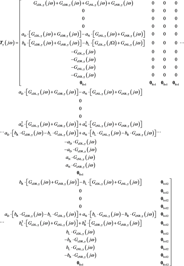(31)

With: $T_{\text{z}}\left(j\omega \right),T_{\text{v}}\left(j\omega \right),T_{\text{a}}\left(j\omega \right)\in {ℂ}^{18\times 18}$ and $T_0\left(j\omega \right)=0_{18}\in {ℝ}^{18\times 18}$ and with the zero-matrix $0_{8\times 12}\in {ℝ}^{8\times 12}$. Now, the output vector $Y_{\gamma }\left(j\omega \right)$ can be calculated by:

$Y_{\text{γ}}\left(j\omega \right)=G_{\text{γ}}\left(j\omega \right)\cdot \left[F_{\text{u}}\left(j\omega \right)+M_{\text{u}}\left(j\omega \right)\right]$ (32)

and the frequency response matrix $G_{\text{γ}}\left(j\omega \right)$ can be written by:

$\begin{array}{l}{G}_{\text{γ}}\left(j\omega \right)={\left[I_{54}+\left(C_{\text{st}}\cdot {\left(I_{36}\cdot j\omega -A_{\text{st}}\right)}^{-1}\cdot B_{\text{st}}+D_{\text{st}}\right)\cdot T_{\text{st},\text{γ}}\right]}^{-1}\\ \cdot \left[C_{\text{st}}\cdot {\left(I_{36}\cdot j\omega -A_{\text{st}}\right)}^{-1}\cdot B_{\text{st}}+D_{\text{st}}\right]\end{array}$ (33)

The frequency response vector for each single kind of excitation can now be derived, with following Fouier-transformations, with the Dirac-delta function $\delta$ :

$\begin{array}{c}{F}_{\text{u}}\left(j\omega \right)=\mathcal{F}\left\{f_{\text{u}}\left(t\right)\right\}=\mathcal{F}\left\{P_{\text{e}}\cdot {\Omega }^2\cdot \underset{u_{\text{e}}}{\underset{︸}{m_{\text{r}}\cdot \hat{e}\cdot e^{j\cdot {\phi }_{\text{e}}}}}\cdot e^{j\cdot \Omega \cdot t}\right\}\\ =P_{\text{e}}\cdot {\Omega }^2\cdot \underset{u_{\text{e}}}{\underset{︸}{m_{\text{r}}\cdot \hat{e}\cdot e^{j\cdot {\phi }_{\text{e}}}}}\cdot 2\pi \cdot \delta \left(\omega -\Omega \right)\end{array}$ (34)

$\begin{array}{c}{M}_{\text{u}}\left(j\omega \right)=\mathcal{F}\left\{m_{\text{u}}\left(t\right)\right\}=\mathcal{F}\left\{P_{\alpha }\cdot {\Omega }^2\cdot \underset{u_{\alpha }}{\underset{︸}{\left({\theta }_{\text{rzy}}-{\theta }_{\text{rx}}\right)\cdot \hat{\alpha }\cdot e^{j\cdot {\phi }_{\alpha }}}}\cdot e^{j\cdot \Omega \cdot t}\right\}\\ =P_{\alpha }\cdot {\Omega }^2\cdot \underset{u_{\alpha }}{\underset{︸}{\left({\theta }_{\text{rzy}}-{\theta }_{\text{rx}}\right)\cdot \hat{\alpha }\cdot e^{j\cdot {\phi }_{\alpha }}}}\cdot 2\pi \cdot \delta \left(\omega -\Omega \right)\end{array}$ (35)

Further on, the index $\kappa$ is used for both kinds of unbalance, representing the excitations:

$\kappa =\text{e},\alpha$ (36)

The output vector $Y_{\text{γ},\text{κ}}\left(j\omega \right)$ for each kind of unbalance can be calculated by:

$Y_{\text{γ},\text{κ}}\left(j\omega \right)=\underset{G_{\text{γ},\text{κ}}\left(j\omega \right)}{\underset{︸}{G_{\text{γ}}\left(j\omega \right)\cdot P_{\text{κ}}\cdot {\Omega }^2}}\cdot u_{\text{κ}}\cdot 2\pi \cdot \delta \left(\omega -\Omega \right)$ (37)

Using the sifting property of the Dirac delta function $\delta \left(\omega -\Omega \right)$, the Fourier-transformed output vector for each kind of unbalance follows:

$Y_{\text{γ},\text{κ}}\left(j\omega \right)=\underset{G_{\text{γ},\text{κ}}\left(j\Omega \right)}{\underset{︸}{G_{\text{γ}}\left(j\Omega \right)\cdot P_{\text{κ}}\cdot {\Omega }^2}}\cdot u_{\text{κ}}\cdot 2\pi \cdot \delta \left(\omega -\Omega \right)$ (38)

Now, the inverse transformation of this Fourier-transformed output vector $Y_{\text{γ},\text{κ}}\left(j\omega \right)$ back into the time-domain can be done:

$\begin{array}{c}{y}_{\text{γ},\text{κ}}\left(t\right)={\mathcal{F}}^{-1}\left\{Y_{\text{γ},\text{κ}}\left(j\omega \right)\right\}={\mathcal{F}}^{-1}\left\{\underset{G_{\text{γ},\text{κ}}\left(j\Omega \right)}{\underset{︸}{G_{\text{γ}}\left(j\Omega \right)\cdot P_{\text{κ}}\cdot {\Omega }^2}}\cdot u_{\text{κ}}\cdot 2\pi \cdot \delta \left(\omega -\Omega \right)\right\}\\ =\underset{{\hat{y}}_{\text{γ},\text{κ}}}{\underset{︸}{\underset{G_{\text{γ},\text{κ}}\left(j\Omega \right)}{\underset{︸}{G_{\text{γ}}\left(j\Omega \right)\cdot P_{\text{κ}}\cdot {\Omega }^2}}\cdot u_{\text{κ}}}}\cdot e^{j\Omega t}\end{array}$ (39)

It is useful to relate the amplitude output vector on the respective unbalance:

${\hat{y}}_{\text{γ},\text{κ},\text{ref}}=\frac{{\hat{y}}_{\text{γ},\text{κ}}}{u_{\text{κ}}}=\underset{G_{\text{γ},\text{κ}}\left(j\Omega \right)}{\underset{︸}{G_{\text{γ}}\left(j\Omega \right)\cdot P_{\text{κ}}\cdot {\Omega }^2}}$ (40)

At this point it is important to mention, that beside the gyroscopic matrix $G$ also the damping matrix $D$ depends on the rotary angular frequency W. The reason is that for forced vibration due to the unbalance, the whirling angular frequency ${\omega }_{\text{F}}$ for the mechanical damping coefficients (8), is equal to the rotary angular frequency W ( ${\omega }_{\text{F}}=\Omega$ ).Therefore, the matrices $A_{\text{st}}$ and $C_{\text{st}}$ are also functions of the rotor angular frequency W. The frequency response matrix $G_{\text{γ}}\left(j\Omega \right)$ can now be formulated by:

$\begin{array}{l}{G}_{\text{γ}}\left(j\Omega \right)={\left[I_{54}+\left(C_{\text{st}}\left(\Omega \right)\cdot {\left(I_{36}\cdot j\Omega -A_{\text{st}}\left(\Omega \right)\right)}^{-1}\cdot B_{\text{st}}+D_{\text{st}}\right)\cdot T_{\text{st},\text{γ}}\left(j\Omega \right)\right]}^{-1}\\ \cdot \left[C_{\text{st}}\left(\Omega \right)\cdot {\left(I_{36}\cdot j\Omega -A_{\text{st}}\left(\Omega \right)\right)}^{-1}\cdot B_{\text{st}}+D_{\text{st}}\right]\end{array}$ (41)

With this matrix, the frequency response vector $G_{\text{γ},\text{κ}}\left(j\Omega \right)$ for both kinds of unbalance can be described:

$G_{\text{γ},\text{κ}}\left(j\Omega \right)=\frac{{\hat{y}}_{\text{γ},\text{κ}}}{u_{\text{κ}}}=G_{\text{γ}}\left(j\Omega \right)\cdot P_{\text{κ}}\cdot {\Omega }^2$ (42)

With this frequency response vector $G_{\text{γ},\text{κ}}\left(j\Omega \right)$ and the kinematic constraints in [22], the response functions for vibration velocities of the bearing housings, and of the foundation points can be derived, as well as the response functions for the actuator forces, based on [22]. The equations are shown in the Appendix.

3.3. Stability Analysis

Due to the use of active vibration control, a stability analysis is very important, therefore the poles of the system have to be derived. Based on [22], the poles can be calculated by solving the following equation:

$\det \left[I_{36}\cdot s-A_{\text{st}}+B_{\text{st}}\cdot T_{\text{st},\text{γ}}\left(s\right)\cdot {\left(I_{54}+D_{\text{st}}\cdot T_{\text{st},\text{γ}}\left(s\right)\right)}^{-1}\cdot C_{\text{st}}\right]=0$ (43)

However, this direct procedure is only possible if the matrices $A_{\text{st}}$ and $C_{\text{st}}$ are independent of the whirling angular frequency ${\omega }_{\text{F}}$, which is here not the case, because the damping coefficients depend here on ${\omega }_{\text{F}}$. The whirling angular frequency ${\omega }_{\text{F}}$ corresponds here—when calculating the pols—to the natural angular frequency and therefore to the imaginary part of the complex poles. Therefore, the use of the damping coefficient lead here to a causality problem. Therefore, a worst case procedure is here derived to investigate the stability of the system. The basic requirements are:

· The mechanical damping of the actuators and the foundation is low, which should be usually the case, so that the mechanical loss factors for the actuators and the foundation fulfill following conditions:

$\tan {\delta }_{\text{aij}}<0.2$ and $\tan {\delta }_{\text{fij}}<0.2$ (44)

· The modal mass of the foundation is so low, that only the first six natural vibration modes have to be taken into account.

· The first six natural vibration modes have conjugate complex poles.

Therefore, following worst case procedure is derived to calculate the pols $s_{\text{n}}$, which is shown in Figure 4. In the first step, the pols are calculated without damping ( $D=0$ ) and with open control loops ( $T_{\text{st},\gamma }\left(s\right)=0$ ).

Then, the natural angular frequency of the 6^th conjugate complex pole pair ${\omega }_6$ —which is set to be equal to the whirling angular frequency ${\omega }_{\text{F}}$ —is considered, for calculating the damping coefficients $d_{\text{aqij}}$ and $d_{\text{fqij}}$. Afterwards, the pols are calculated again, considering damping ( $D\ne 0$ ) and the closed control loop operation ( $T_{\text{st},\gamma }\left(s\right)\ne 0$ ). The corresponding conjugate complex pol pair $s_6^{*}$ is again taken into account for deriving the new damping coefficients. Finally the pols are calculated with the modified damping matrix $D$. If the change of the whirling angular frequency is too large (e.g. more than 5%) this approach can be repeated in loops. This procedure presents a worst case scenario regarding instability, because the natural angular frequency of the highest considerable mode (here mode 6) is used for calculating the damping coefficients, which lead to the

lowest damping coefficients.

Figure 4. Flow diagram for calculating the pols of the vibration system.

3.4. Mathematical Description for Special Controllers

In this section, special controllers—standard controllers (P-, I-, PI-, PD-(ideal), PID-(ideal) controllers)—are analyzed. Therefore, the control parameter can now be directly implemented into the mass matrix and/or the damping matrix and/or the stiffness matrix, which can be seen in Figure 5, referring to [22].

Therefore, the differential equation can be described now by:

$\tilde{M}\cdot \ddot{q}+\left(\tilde{D}+G\right)\cdot \stackrel{\dot{}}{q}+\tilde{C}\cdot q=f_{\text{u}}+m_{\text{u}}$ (45)

By implementing the control parameters into the mass matrix, $\tilde{M}$ becomes $M_{\text{con}}$. When they are implemented into the damping matrix, $\tilde{D}$ becomes $D_{\text{con}}$, and if they are implemented into the stiffness matrix, $\tilde{C}$ becomes $C_{\text{con}}$. The structure of these matrices is shown in (49). Following definitions are used, referring to [22]:

For the mass matrix $C_{\text{con}}$ : $M_{\text{con}}={\Psi }_{\text{con}}$ and $\psi =m$ (46)

For the damping matrix $D_{\text{con}}$ : $D_{\text{con}}={\Psi }_{\text{con}}$ and $\psi =d$ (47)

For the stiffness matrix $C_{\text{con}}$ : $C_{\text{con}}={\Psi }_{\text{con}}$ and $\psi =c$ (48)

The matrices with the integrated controller parameters are formulated by:

Figure 5. Matrices, depending on standard controller structures and different feedback strategies, referring to [22].

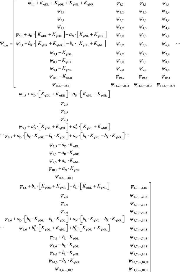(49)

The controller parameters $K_{\text{ψij}}$ depend on the controller structure and the chosen feedback strategy (Figure 5). The combination in Figure 5 marked with “¾” cannot be deduced, if the differential equation system (45) shall be used. If the control parameters are identical, the cells with identical color lead to the same differential equation. The inhomogeneous differential equation (45) can now be solved, based on the common approach.

4. Numerical Example

Now, a numerical example is presented, where the vibration stability, as well as the forced vibrations of a rotating machine are analyzed.

4.1. Boundary Conditions

The data of the rotating machine are shown in Table 1. As it can be seen, the rotating machine has a symmetrical machine design (b_L = b_R; a_D = a_N).

The foundation is a simplified steel frame foundation, which consists of two I-beams (green), which are stiffened by additional welded steel sheets (brown) in the area of the machine feet (cyan), and fixed (red) to ground (Figure 6). No

Table 1. Data of the rotating machine.

Figure 6. Simplified model of the steel frame foundation.

stiffening effect in the area of the machine feet is considered, so that a low stiffness of the steel frame foundation is considered here, as a worst case.

The substitute foundation stiffness, which is necessary to use the model in Table 2, is derived by a finite element analysis of the foundation, but still presenting a simplification.

In this example only three actuators are used, two on drive-side, left and right (DL, DR) and only one actuator on non-drive side left (NL) (Table 3). The fourth actuator on the non-drive side right (NR) is exchanged by a stiff element.

The data of the stiff element is shown in Table 4.

For the control system, I-controllers with feedbacks of the vertical machine feet accelerations are chosen, so that following controller transfer function is used.

$G_{\text{cji},\text{a}}\left(s\right)=\frac{b_{0,\text{ij},\text{a}}}{s}$ (50)

Table 2. Data of the foundation.

Table 3. Data of the actutaors on position DL, DR and NL.

Table 4. Data of the stiff element on position NR.

Table 5. Data of the controller parameters.

The data of the control parameters are shown in Table 5. All three controllers—for the three actuators—have identical parameters. The control parameter for the fourth controller on NR has to be set to zero, because here a stiff element is used instead of an actuator.

Afterwards three different cases are analyzed:

· Case 1: The rotating machine is directly mounted on the steel frame foundation.

· Case 2: Three actuators at DL, DR, NL and a stiff element at NR are placed between machine feet and foundation. The actuators are only operating passively (open control loops).

· Case 3: Same setting as case 2, but the actuators are now operating actively (closed control loops).

4.2. Stability Analysis

To analyze the stability of the system, the poles are calculated for the three different cases, based on the procedure, described in Figure 4. It can be clearly shown, that for all three cases vibration stability exists, because all characteristic poles have no positive real parts (Figure 7, Figure 8 and Figure 9).

When comparing the figures, it is obvious that the damping of the poles can be strongly increased by the active vibration control system (case 3), compared to case 1 and case 2.

4.3. Frequency Response Analysis

Now, the amplitudes of the frequency response functions of bearing housing vibration velocities and of foundation vibration velocities are computed, as well as the frequency response functions of the actuator forces, all related to the respective unbalance. The amplitudes of the frequency response functions are calculated in [dB] with the reference gauge in Si-Unit, in a frequency range from 1 Hz to 250 Hz. An additional index d is now introduced for case 1, so that now following definitions are used:

$\gamma =0,z,v,a,d;i=D,N;j=L,R;q=x,y,z;\kappa =e,\alpha$ (51)

Related bearing housing vibration velocities:

Figure 7. Poles for case 1, calculated at rotational frequency $f_{\text{r}}=0\text{Hz}$ and $f_{\text{r}}=250\text{Hz}$.

Figure 8. Poles for case 2, calculated at rotational frequency $f_{\text{r}}=0\text{Hz}$ and $f_{\text{r}}=250\text{Hz}$.

Figure 9. Poles for case 3, calculated at rotational frequency $f_{\text{r}}=0\text{Hz}$ and $f_{\text{r}}=250\text{Hz}$.

${\left|G_{\text{γ},\text{<mover accent="true"> <mi> v </mi> <mo> ^ </mo> </mover> biq},\text{κ}}\left(j\Omega \right)\right|}_{\text{dB}}=20\cdot \log \left(\frac{\left|G_{\text{γ},\text{<mover accent="true"> <mi> v </mi> <mo> ^ </mo> </mover> biq},\text{κ}}\left(j\Omega \right)\right|}{{\left|G_{\text{γ},\text{<mover accent="true"> <mi> v </mi> <mo> ^ </mo> </mover> biq},\text{κ}}\left(j\Omega \right)\right|}_{\text{ref}}}\right)$ (52)

with: ${\left|G_{\text{γ},\text{<mover accent="true"> <mi> v </mi> <mo> ^ </mo> </mover> biq},\text{κ}}\left(j\Omega \right)\right|}_{\text{ref}}=\{\begin{array}{l}1\frac{\text{m}/\text{s}}{\text{kg}\cdot \text{m}}\text{for}\kappa =e\\ 1\frac{\text{m}/\text{s}}{\text{kg}\cdot {\text{m}}^2}\text{for}\kappa =\alpha \end{array}$

Related foundation vibration velocities:

${\left|G_{\text{γ},\text{<mover accent="true"> <mi> v </mi> <mo> ^ </mo> </mover> fijq},\text{κ}}\left(j\Omega \right)\right|}_{\text{dB}}=20\cdot \log \left(\frac{\left|G_{\text{γ},\text{<mover accent="true"> <mi> v </mi> <mo> ^ </mo> </mover> fijq},\text{κ}}\left(j\Omega \right)\right|}{{\left|G_{\text{γ},\text{<mover accent="true"> <mi> v </mi> <mo> ^ </mo> </mover> fijq},\text{κ}}\left(j\Omega \right)\right|}_{\text{ref}}}\right)$ (53)

with: ${\left|G_{\text{γ},\text{<mover accent="true"> <mi> v </mi> <mo> ^ </mo> </mover> fijq},\text{κ}}\left(j\Omega \right)\right|}_{\text{ref}}=\{\begin{array}{l}1\frac{\text{m}/\text{s}}{\text{kg}\cdot \text{m}}\text{for}\kappa =e\\ 1\frac{\text{m}/\text{s}}{\text{kg}\cdot {\text{m}}^2}\text{for}\kappa =\alpha \end{array}$

Related actuator forces:

${\left|G_{\text{γ},\text{<mover accent="true"> <mi> f </mi> <mo> ^ </mo> </mover> azij},\text{κ}}\left(j\Omega \right)\right|}_{\text{dB}}=20\cdot \log \left(\frac{\left|G_{\text{γ},\text{<mover accent="true"> <mi> f </mi> <mo> ^ </mo> </mover> azij},\text{κ}}\left(j\Omega \right)\right|}{{\left|G_{\text{γ},\text{<mover accent="true"> <mi> f </mi> <mo> ^ </mo> </mover> azij},\text{κ}}\left(j\Omega \right)\right|}_{\text{ref}}}\right)$ (54)

with: ${\left|G_{\text{γ},\text{<mover accent="true"> <mi> f </mi> <mo> ^ </mo> </mover> azij},\text{κ}}\left(j\Omega \right)\right|}_{\text{ref}}=\{\begin{array}{l}1\frac{\text{N}}{\text{kg}\cdot \text{m}}\text{for}\kappa =e\\ 1\frac{\text{N}}{\text{kg}\cdot {\text{m}}^2}\text{for}\kappa =\alpha \end{array}$

4.3.1. Excitation by Static Unbalance

The amplitude response functions for the bearing housing vibration velocities at the drive side and at the non-drive side, related to static unbalance are shown in Figure 10.

The amplitude response functions for the foundation vibration velocities at the drive side, related to static unbalance are shown in Figure 11.

The amplitude response functions for the foundation vibration velocities at the non-drive side, related to static unbalance are shown in Figure 12.

The frequency response functions for the actuator forces, related to static

Figure 10. Amplitude response functions for the bearing housing vibration velocities at the drive side and at the non-drive side, related to static unbalance $u_{\text{e}}$ for case 1, case 2 and case 3.

Figure 11. Amplitude response functions for the foundation vibration velocities at the drive side (left and right), related to static unbalance $u_{\text{e}}$ for case 1, case 2 and case 3.

Figure 12. Amplitude response functions for the foundation vibration velocities at the non-drive side (left and right), related to static unbalance $u_{\text{e}}$ for case 1, case 2 and case 3.

Figure 13. Frequency response functions for the actuator forces, related to static unbalance $u_{\text{e}}$ (case 3) at drive side left (DL), drive side right (DR), non-drive side left (NL) and non-drive side right (NR).

unbalance are shown in Figure 13.

4.3.2. Excitation by Moment Unbalance

The amplitude response functions for the bearing housing vibration velocities at the drive side and at the non-drive side, related to moment unbalance are shown in Figure 14.

The amplitude response functions for the foundation vibration velocities at the drive side, related to moment unbalance are shown in Figure 15.

The amplitude response functions for the foundation vibration velocities at the non-drive side, related to moment unbalance are shown in Figure 16.

The frequency response functions for the actuator forces, related to moment unbalance are shown in Figure 17.

4.3.3. Discussion of the Frequency Response Analysis

The amplitude response functions for the bearing housing vibration velocities

Figure 14. Amplitude response functions for the bearing housing vibration velocities on the drive side and on the non-drive side, related to moment unbalance $u_{\alpha }$ for case 1, case 2 and case 3.

Figure 15. Amplitude response functions for the foundation vibration velocities at the drive side (left and right), related to moment unbalance $u_{\alpha }$ for case 1, case 2 and case 3.

Figure 16. Amplitude response functions for the foundation vibration velocities at the non-drive side (left and right), related to moment unbalance $u_{\alpha }$ for case 1, case 2 and case 3.

Figure 17. Frequency response functions for the actuator forces, related to moment unbalance $u_{\alpha }$ (case 3) at drive side left (DL), drive side right (DR), non-drive side left (NL) and non-drive side right (NR).

for excitation by a static unbalance (Figure 10) show, that in the analyzed rotational frequency range two resonance frequencies occur for case 1—where the machine is directly mounted on the steel frame foundation—at about $f_{\text{r}}=38.1\text{Hz}$ and at $f_{\text{r}}=126.4\text{Hz}$. Figure 10 shows additionally, that no axial vibrations occur for case 1, if only a static unbalance is considered. For a moment unbalance, three resonance frequencies occur for case 1, at about $f_{\text{r}}=82.8\text{Hz}$, $f_{\text{r}}=110.5\text{Hz}$ and $f_{\text{r}}=198.5\text{Hz}$ (Figure 14). The natural mode, where the machine mass is mainly rotating at the x-axis—with a natural angular frequency of about 1088 rad/s (Figure 7), which means a natural frequency of about 173, 2 Hz—leads not to a resonance regarding bearing housing vibrations, because this mode shape is hardly excited by these two kinds of unbalance. Because of the symmetrical machine design and the identical foundation stiffness and damping coefficient under each machine feet, the frequency response functions for the bearing housing vibration velocities are identical for the drive side and the non-drive side for case 1. If now the machine is mounted on a stiff element and on three actuators, operating with open control loops (case 2), the resonance frequencies for the bearing housing vibrations occur at lower frequencies and six different resonance frequencies are obvious, when considering both kind of unbalance (Figure 10 and Figure 14). The amplitudes in the resonance frequencies are clearly lower for case 2 compared to amplitudes in the resonance frequencies for case 1, because the amplitudes of excitation force and of the excitation moment are proportional to $f_{\text{r}}^2$. When now the control loops are closed— which means case 3—most of the resonances regarding the related bearing housing vibrations (Figure 10 and Figure 14) get well damped—as well as most of the related foundation vibrations (Figure 11, Figure 12, Figure 15, Figure 16), when comparing the red curves with the blue curves. Therefore, an operation in the rotational frequency range from 0 Hz to 80 Hz seems now possible for case 3, without off-limits areas regarding rotational frequency. If the machine would be mounted directly on the foundation (case 1), this would not be possible, because a sharp resonance at 38.1 Hz occurs here due to static unbalance, regarding the related bearing housing vibrations (Figure 10) and regarding the related foundation vibrations (Figure 11 and Figure 12). Figure 13 and Figure 17 show the frequency response functions regarding the active actuator forces. It can be seen, that with increasing rotational frequency also the amplitudes of the actuator force frequency response functions increase, because the unbalance force and unbalance moment also increase with the rotational frequency. Of course, the actuator forces are also strongly influenced by the vibration mode shapes. No active actuator force occurs on position NR, because a stiff element is positioned there instead of an actuator. If the stiff element would be exchanged by a fourth actuator, so that four identical actuators would be used—case 2 gets case 2* and case 3 gets case 3* (with four identical control parameters)—a symmetrical system would exist. With such a symmetrical system, a vibration mode exists, where the machine makes a pure rotating at the z-axis. This mode cannot be influenced by the actuators anymore, because they are only acting in vertical direction. This is shown in Figure 18 regarding the amplitude response functions for the bearing housing vibration velocities in horizontal direction. The resonance frequency at about 18.6 Hz cannot be damped by the control system. Only a marginal difference between the blue curve and the red curve for horizontal direction

Figure 18. Amplitude response functions for the bearing housing vibration velocities on the drive side and on the non-drive side, related to moment unbalance $u_{\alpha }$ for case 1, case 2* and case 3* (*: Four identical actuators are used).

is obvious in Figure 18, which is caused by the gyroscopic effect, leading here to a marginal coupling of the vibration modes, so that no absolute pure vibration mode at the z-axis occurs. Because of the symmetrical system, the frequency response functions for the bearing housing vibration velocities are now identical for drive side and non-drive side (Figure 18).

Therefore, it could be shown, that the method “vibration mode coupling by asymmetry”, which was developed and mathematically described in [22] for a rigid foundation, is also transferable for a soft foundation.

5. Conclusion

The paper presents a simplified 3D-model for active vibration control of rotating machines with active machine foot mounts on soft foundations, considering static and moment unbalance. After the model was mathematical described in the time domain, it was transferred into the Fourier domain, where the frequencies response functions regarding bearing housing vibrations, foundation vibrations and actuator forces have been derived. Afterwards, the mathematical coherences have been described in the Laplace domain and a worst case procedure was derived to analyze the vibration stability. For special controller structures in combination with certain feedback strategies, a calculation method was shown, where the controller parameters can directly be implemented into the stiffness matrix, damping matrix and mass matrix. Additionally a numerical example was presented, where the vibration stability and the frequency response functions have been analyzed. It could be shown, that with the active vibration control system all vibration modes can be damped well, so that an operation in the rotational frequency range from 0 Hz to 80 Hz is possible without off-limits areas.

Finally it could be demonstrated, that the method “vibration mode coupling by asymmetry”, which was developed and mathematically described in [22] for a rigid foundation, is also transferable for soft foundations. The numerical example was also used, to validate the presented model with a finite element analysis by comparing the results. However also a validation by measurement is planned. Therefore, a test bed for an 11 kW induction motor, mounted on a soft steel frame foundation with actuators, has been built and first experimental investigations have been deduced [23], showing good congruence with the presented 3D-model.

Appendix:

A1. Coefficients of the Matrices

Coefficients of the mass matrix M:

$m_{1,1}=m_{2,2}=m_{3,3}=m_{\text{sr}}+m_{\text{aaDL}}+m_{\text{aaDR}}+m_{\text{aaNL}}+m_{\text{aaNR}}$ (55)

$m_{1,5}=m_{5,1}=a_{\text{D}}\cdot \left(m_{\text{aaDL}}+m_{\text{aaDR}}\right)-a_{\text{N}}\cdot \left(m_{\text{aaNL}}+m_{\text{aaNR}}\right)$ (56)

$m_{1,6}=m_{6,1}=b_{\text{R}}\cdot \left(m_{\text{aaDR}}+m_{\text{aaNR}}\right)-b_{\text{L}}\cdot \left(m_{\text{aaDL}}+m_{\text{aaNL}}\right)$ (57)

$m_{2,4}=m_{4,2}=-a_{\text{D}}\cdot \left(m_{\text{aaDL}}+m_{\text{aaDR}}\right)+a_{\text{N}}\cdot \left(m_{\text{aaNL}}+m_{\text{aaNR}}\right)$ (58)

$m_{2,6}=m_{6,2}=-h\cdot \left(m_{\text{aaDL}}+m_{\text{aaDR}}+m_{\text{aaNL}}+m_{\text{aaNR}}\right)$ (59)

$m_{3,4}=m_{4,3}=-b_{\text{R}}\cdot \left(m_{\text{aaDR}}+m_{\text{aaNR}}\right)+b_{\text{L}}\cdot \left(m_{\text{aaDL}}+m_{\text{aaNL}}\right)$ (60)

$m_{3,5}=m_{5,3}=h\cdot \left(m_{\text{aaDL}}+m_{\text{aaDR}}+m_{\text{aaNL}}+m_{\text{aaNR}}\right)$ (61)

$\begin{array}{l}{m}_{4,4}={\theta }_{\text{srz}}+b_{\text{L}}^2\cdot \left(m_{\text{aaDL}}+m_{\text{aaNL}}\right)+b_{\text{R}}^2\cdot \left(m_{\text{aaDR}}+m_{\text{aaNR}}\right)\\ +a_{\text{D}}^2\cdot \left(m_{\text{aaDL}}+m_{\text{aaDR}}\right)+a_{\text{N}}^2\cdot \left(m_{\text{aaNL}}+m_{\text{aaNR}}\right)\end{array}$ (62)

$m_{4,5}=m_{5,4}=h\cdot b_{\text{L}}\cdot \left(m_{\text{aaDL}}+m_{\text{aaNL}}\right)-h\cdot b_{\text{R}}\cdot \left(m_{\text{aaDR}}+m_{\text{aaNR}}\right)$ (63)

$m_{4,6}=m_{6,4}=h\cdot a_{\text{D}}\cdot \left(m_{\text{aaDL}}+m_{\text{aaDR}}\right)-h\cdot a_{\text{N}}\cdot \left(m_{\text{aaNL}}+m_{\text{aaNR}}\right)$ (64)

$\begin{array}{c}{m}_{5,5}={\theta }_{\text{sry}}+a_{\text{D}}^2\cdot \left(m_{\text{aaDL}}+m_{\text{aaDR}}\right)+a_{\text{N}}^2\cdot \left(m_{\text{aaNL}}+m_{\text{aaNR}}\right)\\ +h^2\cdot \left(m_{\text{aaDL}}+m_{\text{aaDR}}+m_{\text{aaNL}}+m_{\text{aaNR}}\right)\end{array}$ (65)

$m_{5,6}=m_{6,5}=a_{\text{D}}\cdot \left(b_{\text{R}}\cdot m_{\text{aaDR}}-b_{\text{L}}\cdot m_{\text{aaDL}}\right)+a_{\text{N}}\cdot \left(b_{\text{L}}\cdot m_{\text{aaNL}}-b_{\text{R}}\cdot m_{\text{aaNR}}\right)$ (66)

$\begin{array}{c}{m}_{6,6}={\theta }_{\text{sx}}+b_{\text{L}}^2\cdot \left(m_{\text{aaDL}}+m_{\text{aaNL}}\right)+b_{\text{R}}^2\cdot \left(m_{\text{aaDR}}+m_{\text{aaNR}}\right)\\ +h^2\cdot \left(m_{\text{aaDL}}+m_{\text{aaDR}}+m_{\text{aaNL}}+m_{\text{aaNR}}\right)\end{array}$ (67)

$m_{7,7}=m_{11,11}=m_{15,15}=m_{\text{fDL}}+m_{\text{asDL}}$ (68)

$m_{8,8}=m_{12,12}=m_{16,16}=m_{\text{fDR}}+m_{\text{asDR}}$ (69)

$m_{9,9}=m_{13,13}=m_{17,17}=m_{\text{fNL}}+m_{\text{asNL}}$ (70)

$m_{10,10}=m_{14,14}=m_{18,18}=m_{\text{fNR}}+m_{\text{asNR}}$ (71)

The other coefficients are zero.

Coefficients of the stiffness matrix C:

$c_{1,1}=c_{\text{azDL}}+c_{\text{azDR}}+c_{\text{azNL}}+c_{\text{azNR}}$ (72)

$c_{1,5}=c_{5,1}=a_{\text{D}}\cdot \left(c_{\text{azDL}}+c_{\text{azDR}}\right)-a_{\text{N}}\cdot \left(c_{\text{azNL}}+c_{\text{azNR}}\right)$ (73)

$c_{1,6}=c_{6,1}=b_{\text{R}}\cdot \left(c_{\text{azDR}}+c_{\text{azNR}}\right)-b_{\text{L}}\cdot \left(c_{\text{azDL}}+c_{\text{azNL}}\right)$ (74)

$c_{1,7}=c_{7,1}=-c_{\text{azDL}}$ (75)

$c_{1,8}=c_{8,1}=-c_{\text{azDR}}$ (76)

$c_{1,9}=c_{9,1}=-c_{\text{azNL}}$ (77)

$c_{1,10}=c_{10,1}=-c_{\text{azNR}}$ (78)

$c_{2,2}=c_{\text{ayDL}}+c_{\text{ayDR}}+c_{\text{ayNL}}+c_{\text{ayNR}}$ (79)

$c_{2,4}=c_{4,2}=a_{\text{N}}\cdot \left(c_{\text{ayNL}}+c_{\text{ayNR}}\right)-a_{\text{D}}\cdot \left(c_{\text{ayDL}}+c_{\text{ayDR}}\right)$ (80)

$c_{2,6}=c_{6,2}=-h\cdot \left(c_{\text{ayDL}}+c_{\text{ayDR}}+c_{\text{ayNL}}+c_{\text{ayNR}}\right)$ (81)

$c_{2,11}=c_{11,2}=-c_{\text{ayDL}}$ (82)

$c_{2,12}=c_{12,2}=-c_{\text{ayDR}}$ (83)

$c_{2,13}=c_{13,2}=-c_{\text{ayNL}}$ (84)

$c_{2,14}=c_{14,2}=-c_{\text{ayNR}}$ (85)

$c_{3,3}=c_{\text{axDL}}+c_{\text{axDR}}+c_{\text{axNL}}+c_{\text{axNR}}$ (86)

$c_{3,4}=c_{4,3}=b_{\text{L}}\cdot \left(c_{\text{axDL}}+c_{\text{axNL}}\right)-b_{\text{R}}\cdot \left(c_{\text{axDR}}+c_{\text{axNR}}\right)$ (87)

$c_{3,5}=c_{5,3}=h\cdot \left(c_{\text{axDL}}+c_{\text{axDR}}+c_{\text{axNL}}+c_{\text{axNR}}\right)$ (88)

$c_{3,15}=c_{15,3}=-c_{\text{axDL}}$ (89)

$c_{3,16}=c_{16,3}=-c_{\text{axDR}}$ (90)

$c_{3,17}=c_{17,3}=-c_{\text{axNL}}$ (91)

$c_{3,18}=c_{18,3}=-c_{\text{axNR}}$ (92)

$\begin{array}{c}{c}_{4,4}=b_{\text{L}}^2\cdot \left(c_{\text{axDL}}+c_{\text{axNL}}\right)+b_{\text{R}}^2\cdot \left(c_{\text{axDR}}+c_{\text{axNR}}\right)\\ +a_{\text{D}}^2\cdot \left(c_{\text{ayDL}}+c_{\text{ayDR}}\right)+a_{\text{N}}^2\cdot \left(c_{\text{ayNL}}+c_{\text{ayNR}}\right)\end{array}$ (93)

$c_{4,5}=c_{5,4}=h\cdot b_{\text{L}}\cdot \left(c_{\text{axDL}}+c_{\text{axNL}}\right)-h\cdot b_{\text{R}}\cdot \left(c_{\text{axDR}}+c_{\text{axNR}}\right)$ (94)

$c_{4,6}=c_{6,4}=h\cdot a_{\text{D}}\cdot \left(c_{\text{ayDL}}+c_{\text{ayDR}}\right)-h\cdot a_{\text{N}}\cdot \left(c_{\text{ayNL}}+c_{\text{ayNR}}\right)$ (95)

$c_{4,11}=c_{11,4}=c_{\text{ayDL}}\cdot a_{\text{D}}$ (96)

$c_{4,12}=c_{12,4}=c_{\text{ayDR}}\cdot a_{\text{D}}$ (97)

$c_{4,13}=c_{13,4}=-c_{\text{ayNL}}\cdot a_{\text{N}}$ (98)

$c_{4,14}=c_{14,4}=-c_{\text{ayNR}}\cdot a_{\text{N}}$ (99)

$c_{4,15}=c_{15,4}=-c_{\text{axDL}}\cdot b_{\text{L}}$ (100)

$c_{4,16}=c_{16,4}=c_{\text{axDR}}\cdot b_{\text{R}}$ (101)

$c_{4,17}=c_{17,4}=-c_{\text{axNL}}\cdot b_{\text{L}}$ (102)

$c_{4,18}=c_{18,4}=c_{\text{axNR}}\cdot b_{\text{R}}$ (103)

$\begin{array}{c}{c}_{5,5}=a_{\text{D}}^2\cdot \left(c_{\text{azDL}}+c_{\text{azDR}}\right)+a_{\text{N}}^2\cdot \left(c_{\text{azNL}}+c_{\text{azNR}}\right)\\ +h^2\cdot \left(c_{\text{axDL}}+c_{\text{axDR}}+c_{\text{axNL}}+c_{\text{axNR}}\right)\end{array}$ (104)

$c_{5,6}=c_{6,5}=a_{\text{D}}\cdot \left(b_{\text{R}}\cdot c_{\text{azDR}}-b_{\text{L}}\cdot c_{\text{azDL}}\right)+a_{\text{N}}\cdot \left(b_{\text{L}}\cdot c_{\text{azNL}}-b_{\text{R}}\cdot c_{\text{azNR}}\right)$ (105)

$c_{5,7}=c_{7,5}=-c_{\text{azDL}}\cdot a_{\text{D}}$ (106)

$c_{5,8}=c_{8,5}=-c_{\text{azDR}}\cdot a_{\text{D}}$ (107)

$c_{5,9}=c_{9,5}=c_{\text{azNL}}\cdot a_{\text{N}}$ (108)

$c_{5,10}=c_{10,5}=c_{\text{azNR}}\cdot a_{\text{N}}$ (109)

$c_{5,15}=c_{15,5}=-c_{\text{axDL}}\cdot h$ (110)

$c_{5,16}=c_{16,5}=-c_{\text{axDR}}\cdot h$ (111)

$c_{5,17}=c_{17,5}=-c_{\text{axNL}}\cdot h$ (112)

$c_{5,18}=c_{18,5}=-c_{\text{axNR}}\cdot h$ (113)

$\begin{array}{c}{c}_{6,6}=b_{\text{L}}^2\cdot \left(c_{\text{azDL}}+c_{\text{azNL}}\right)+b_{\text{R}}^2\cdot \left(c_{\text{azDR}}+c_{\text{azNR}}\right)\\ +h^2\cdot \left(c_{\text{ayDL}}+c_{\text{ayDR}}+c_{\text{ayNL}}+c_{\text{ayNR}}\right)\end{array}$ (114)

$c_{6,7}=c_{7,6}=c_{\text{azDL}}\cdot b_{\text{L}}$ (115)

$c_{6,8}=c_{8,6}=-c_{\text{azDR}}\cdot b_{\text{R}}$ (116)

$c_{6,9}=c_{9,6}=c_{\text{azNL}}\cdot b_{\text{L}}$ (117)

$c_{6,10}=c_{10,6}=-c_{\text{azNR}}\cdot b_{\text{R}}$ (118)

$c_{6,11}=c_{11,6}=c_{\text{ayDL}}\cdot h$ (119)

$c_{6,12}=c_{12,6}=c_{\text{ayDR}}\cdot h$ (120)

$c_{6,13}=c_{13,6}=c_{\text{ayNL}}\cdot h$ (121)

$c_{6,14}=c_{14,6}=c_{\text{ayNR}}\cdot h$ (122)

$c_{7,7}=c_{\text{fzDL}}+c_{\text{azDL}}$ (123)

$c_{8,8}=c_{\text{fzDR}}+c_{\text{azDR}}$ (124)

$c_{9,9}=c_{\text{fzNL}}+c_{\text{azNL}}$ (125)

$c_{10,10}=c_{\text{fzNR}}+c_{\text{azNR}}$ (126)

$c_{11,11}=c_{\text{fyDL}}+c_{\text{ayDL}}$ (127)

$c_{12,12}=c_{\text{fyDR}}+c_{\text{ayDR}}$ (128)

$c_{13,13}=c_{\text{fyNL}}+c_{\text{ayNL}}$ (129)

$c_{14,14}=c_{\text{fyNR}}+c_{\text{ayNR}}$ (130)

$c_{15,15}=c_{\text{fxDL}}+c_{\text{axDL}}$ (131)

$c_{16,16}=c_{\text{fxDR}}+c_{\text{axDR}}$ (132)

$c_{17,17}=c_{\text{fxNL}}+c_{\text{axNL}}$ (133)

$c_{18,18}=c_{\text{fxNR}}+c_{\text{axNR}}$ (134)

The other coefficients are zero.

Coefficients of the damping matrix D:

The coefficients of the damping matrix can be easily derived by just replacing “c” in the formulas (72)-(134) by “d”.

A2. Response Functions for the Bearing Housing Vibration Velocities

· In vertical direction:

Drive side: $G_{\text{γ},\text{<mover accent="true"> <mi> v </mi> <mo> ^ </mo> </mover> bDz},\text{κ}}\left(j\Omega \right)=G_{\text{γ},\text{κ}}{\left(j\Omega \right)}_{19}+l_{\text{D}}\cdot G_{\text{γ},\text{κ}}{\left(j\Omega \right)}_{23}$ (135)

Non-drive side: $G_{\text{γ},\text{<mover accent="true"> <mi> v </mi> <mo> ^ </mo> </mover> bNz},\text{κ}}\left(j\Omega \right)=G_{\text{γ},\text{κ}}{\left(j\Omega \right)}_{19}-l_N\cdot G_{\text{γ},\text{κ}}{\left(j\Omega \right)}_{23}$ (136)

· In horizontal direction:

Drive side: $G_{\text{γ},\text{<mover accent="true"> <mi> v </mi> <mo> ^ </mo> </mover> bDy},\text{κ}}\left(j\Omega \right)=G_{\text{γ},\text{κ}}{\left(j\Omega \right)}_{20}-l_{\text{D}}\cdot G_{\text{γ},\text{κ}}{\left(j\Omega \right)}_{22}$ (137)

Non-drive side: $G_{\text{γ},\text{<mover accent="true"> <mi> v </mi> <mo> ^ </mo> </mover> bNy},\text{κ}}\left(j\Omega \right)=G_{\text{γ},\text{κ}}{\left(j\Omega \right)}_{20}+l_N\cdot G_{\text{γ},\text{κ}}{\left(j\Omega \right)}_{22}$ (138)

· In axial direction:

Drive side: $G_{\text{γ},\text{<mover accent="true"> <mi> v </mi> <mo> ^ </mo> </mover> bDx},\text{κ}}\left(j\Omega \right)=G_{\text{γ},\text{κ}}{\left(j\Omega \right)}_{21}$ (139)

Non-drive side: $G_{\text{γ},\text{<mover accent="true"> <mi> v </mi> <mo> ^ </mo> </mover> bNx},\text{κ}}\left(j\Omega \right)=G_{\text{γ},\text{κ}}{\left(j\Omega \right)}_{21}$ (140)

The element $G_{\text{γ},\text{κ}}{\left(j\Omega \right)}_{\text{n}}$ is the n^th element of the frequency response vector $G_{\text{γ},\text{κ}}\left(j\Omega \right)$.

A3. Response Functions for the Foundation Points Velocities

· In vertical direction:

Drive side, left: $G_{\text{γ},\text{<mover accent="true"> <mi> v </mi> <mo> ^ </mo> </mover> fDLz},\text{κ}}\left(j\Omega \right)=G_{\text{γ},\text{κ}}{\left(j\Omega \right)}_{25}$ (141)

Drive side right: $G_{\text{γ},\text{<mover accent="true"> <mi> v </mi> <mo> ^ </mo> </mover> fDRz},\text{κ}}\left(j\Omega \right)=G_{\text{γ},\text{κ}}{\left(j\Omega \right)}_{26}$ (142)

Non-drive side, left: $G_{\text{γ},\text{<mover accent="true"> <mi> v </mi> <mo> ^ </mo> </mover> fNLz},\text{κ}}\left(j\Omega \right)=G_{\text{γ},\text{κ}}{\left(j\Omega \right)}_{27}$ (143)

Non-drive side, right: $G_{\text{γ},\text{<mover accent="true"> <mi> v </mi> <mo> ^ </mo> </mover> fNRz},\text{κ}}\left(j\Omega \right)=G_{\text{γ},\text{κ}}{\left(j\Omega \right)}_{28}$ (144)

· In horizontal direction:

Drive side, left: $G_{\text{γ},\text{<mover accent="true"> <mi> v </mi> <mo> ^ </mo> </mover> fDLy},\text{κ}}\left(j\Omega \right)=G_{\text{γ},\text{κ}}{\left(j\Omega \right)}_{29}$ (145)

Drive side right: $G_{\text{γ},\text{<mover accent="true"> <mi> v </mi> <mo> ^ </mo> </mover> fDRy},\text{κ}}\left(j\Omega \right)=G_{\text{γ},\text{κ}}{\left(j\Omega \right)}_{30}$ (146)

Non-drive side, left: $G_{\text{γ},\text{<mover accent="true"> <mi> v </mi> <mo> ^ </mo> </mover> fNLy},\text{κ}}\left(j\Omega \right)=G_{\text{γ},\text{κ}}{\left(j\Omega \right)}_{31}$ (147)

Non-drive side, right: $G_{\text{γ},\text{<mover accent="true"> <mi> v </mi> <mo> ^ </mo> </mover> fNRy},\text{κ}}\left(j\Omega \right)=G_{\text{γ},\text{κ}}{\left(j\Omega \right)}_{32}$ (148)

· In axial direction:

Drive side, left: $G_{\text{γ},\text{<mover accent="true"> <mi> v </mi> <mo> ^ </mo> </mover> fDLx},\text{κ}}\left(j\Omega \right)=G_{\text{γ},\text{κ}}{\left(j\Omega \right)}_{33}$ (149)

Drive side right: $G_{\text{γ},\text{<mover accent="true"> <mi> v </mi> <mo> ^ </mo> </mover> fDRx},\text{κ}}\left(j\Omega \right)=G_{\text{γ},\text{κ}}{\left(j\Omega \right)}_{34}$ (150)

Non-drive side, left: $G_{\text{γ},\text{<mover accent="true"> <mi> v </mi> <mo> ^ </mo> </mover> fNLx},\text{κ}}\left(j\Omega \right)=G_{\text{γ},\text{κ}}{\left(j\Omega \right)}_{35}$ (151)

Non-drive side, right: $G_{\text{γ},\text{<mover accent="true"> <mi> v </mi> <mo> ^ </mo> </mover> fNRx},\text{κ}}\left(j\Omega \right)=G_{\text{γ},\text{κ}}{\left(j\Omega \right)}_{36}$ (152)

A4. Response Functions for the Actuator Forces

Feedback of the motor feet displacements $\gamma =z$ :

· For drive side, left:

$G_{\text{γ},\text{<mover accent="true"> <mi> f </mi> <mo> ^ </mo> </mover> azDL},\text{κ}}\left(j\Omega \right)=-\left[G_{\text{γ},\text{κ}}{\left(j\Omega \right)}_1-b_{\text{L}}\cdot G_{\text{γ},\text{κ}}{\left(j\Omega \right)}_6+a_{\text{D}}\cdot G_{\text{γ},\text{κ}}{\left(j\Omega \right)}_5\right]\cdot G_{\text{cDL},\text{γ}}\left(j\Omega \right)$ (153)

· For drive side, right:

$G_{\text{γ},\text{<mover accent="true"> <mi> f </mi> <mo> ^ </mo> </mover> azDR},\text{κ}}\left(j\Omega \right)=-\left[G_{\text{γ},\text{κ}}{\left(j\Omega \right)}_1+b_{\text{R}}\cdot G_{\text{γ},\text{κ}}{\left(j\Omega \right)}_6+a_{\text{D}}\cdot G_{\text{γ},\text{κ}}{\left(j\Omega \right)}_5\right]\cdot G_{\text{cDR},\text{γ}}\left(j\Omega \right)$ (154)

· For non-drive side, left:

$G_{\text{γ},\text{<mover accent="true"> <mi> f </mi> <mo> ^ </mo> </mover> azNL},\text{κ}}\left(j\Omega \right)=-\left[G_{\text{γ},\text{κ}}{\left(j\Omega \right)}_1-b_{\text{L}}\cdot G_{\text{γ},\text{κ}}{\left(j\Omega \right)}_6-a_{\text{N}}\cdot G_{\text{γ},\text{κ}}{\left(j\Omega \right)}_5\right]\cdot G_{\text{cNL},\text{γ}}\left(j\Omega \right)$ (155)

· For non-drive side, right:

$G_{\text{γ},\text{<mover accent="true"> <mi> f </mi> <mo> ^ </mo> </mover> azNR},\text{κ}}\left(j\Omega \right)=-\left[G_{\text{γ},\text{κ}}{\left(j\Omega \right)}_1+b_{\text{R}}\cdot G_{\text{γ},\text{κ}}{\left(j\Omega \right)}_6-a_{\text{N}}\cdot G_{\text{γ},\text{κ}}{\left(j\Omega \right)}_5\right]\cdot G_{\text{cNR},\text{γ}}\left(j\Omega \right)$ (156)

For feedback of the motor feet velocities, index $\gamma$ gets v ( $\gamma =v$ ) and the index number n of the elements $G_{\text{γ},\text{κ}}{\left(j\Omega \right)}_{\text{n}}$ in (153)-(156) has to be changed to $n\to n+18$. For feedback of motor feet accelerations index $\gamma$ gets a ( $\gamma =a$ ) and the index number n of the elements $G_{\text{γ},\text{κ}}{\left(j\Omega \right)}_{\text{n}}$ in (153)-(156) has to be changed to $n\to n+36$. For open loop operation index $\gamma$ gets 0 ( $\gamma =0$ ), and the response functions of the actuator forces are zero.

Conflicts of Interest

The author declares no conflicts of interest regarding the publication of this paper.

References

[1]	Vance, J.M., Zeidan, F.J. and Murphy, B. (2010) Machinery Vibration and Rotordynamics. John Wiley & Sons, Hoboken, 71-118. https://doi.org/10.1002/9780470903704
[2]	Friswell, M.I., Penny, J.E.T., Garvey, S.D. and Lees, A.W. (2010) Dynamics of Rotating Machines. Cambridge University Press, Cambridge, 228-291. https://doi.org/10.1017/CBO9780511780509
[3]	Rao, J.S. (1996) Rotor Dynamics. John Wiley & Sons, New York, 69-312.
[4]	Gasch, R., Nordmann, R. and Pfützner, H. (2002) Rotordynamik. Springer, Berlin-Heidelberg, 17-307. https://doi.org/10.1007/3-540-33884-5
[5]	Gasch, R., Maurer, J. and Sarfeld, W. (1984) The Influence of the Elastic Half Space on Stability and Unbalance of a Simple Rotor-Bearing Foundation System. Proceedings of Conference Vibration in Rotating Machinery, C 300/84, Edinburg, 1-12.
[6]	Kirk, R.G., DeChowdhury, P. and Gunter, E.J. (1974) The Effect of Support Flexibility on the Stability of Rotors Mounted in Plain Cylindrical Bearings. Proceedings IUTAM Symposium Dynamics of Rotors, Lyngby, 244-298. https://doi.org/10.1007/978-3-642-48784-2_11
[7]	Werner, U. (2017) Influence of the Foundation on the Threshold of Stability for Rotating Machines with Roller Bearings—A Theoretical Analysis. JAMP Journal of Applied Mathematics and Physics, 5, 1380-1397. https://doi.org/10.4236/jamp.2017.56114
[8]	Schweitzer, G. and Maslen, E.H. (2009) Magnetic Bearings. Springer, Berlin, 27-433.
[9]	Preumont, A. (2011) Vibration Control of Active Structures: An Introduction. Springer, Berlin, 41-357. https://doi.org/10.1007/978-94-007-2033-6_3
[10]	Janschek, K. (2012) Mechatronic Systems Design: Methods, Models, Concepts. Springer, Berlin, 277-724. https://doi.org/10.1007/978-3-642-17531-2_5
[11]	Ehmann, C. and Nordmann, R. (2012) Comparison of Control Strategies for Active Vibration Control of Flexible Structures. Archives of Control Sciences, 13, 303-312.
[12]	Ushijima, T. and Kumakawa, S. (1993) Active Engine Mount with Piezo-Actuator for Vibration Control. SAE Technical Paper 930201. https://doi.org/10.4271/930201
[13]	Ulbrich, H. (1994) A Comparison of Different Actuator Concepts for Applications in Rotating Machinery. International Journal of Rotating Machinery, 1, 61-71. https://doi.org/10.1155/S1023621X94000060
[14]	Sun, W., Gao, H. and Yao, B. (2013) Adaptive Robust Vibration Control of Full-Car Active Suspensions with Electrohydraulic Actuators. IEEE Transactions on Control Systems Technology, 21, 2417-2422. https://doi.org/10.1109/TCST.2012.2237174
[15]	Sohn, J., Paeng, Y. and Choi, S. (2010) An Active Mount Using an Electromagnetic Actuator for Vibration Control: Experimental Investigation. Proceedings of the Institution of Mechanical Engineers, Part C: Journal of Mechanical Engineering Science, 224, 1617-1625. https://doi.org/10.1243/09544062JMES1902
[16]	Zhang, H., Shi, W., Ke, J., Feng, G., Qu, J. and Chen, Z. (2020) A Review on Model and Control of Electromagnetic Active Engine Mounts. Shock and Vibration, 2020, Article ID: 4289281. https://doi.org/10.1155/2020/4289281
[17]	Fairman, F.W. (1998) Linear Control Theory: The State Space Approach. John Wily and Sons, Hoboken, 1-66.
[18]	Unbehauen, H. (2007) Regelungstechnik II, Zustandsregelungen, digitale und nichtlineare Regelsysteme. Vieweg+Teubner, Vieweg, 1-100.
[19]	Hendricks, E., Jannerup, O. and Haase, P. (2008) Linear Systems Control: Deterministic and Stochastic Methods. Springer, Berlin, 9-291.
[20]	Yedavalli, R.K. (2014) Robust Control of Uncertain Dynamic Systems: A Linear State Space Approach. Springer, Berlin, 13-143. https://doi.org/10.1007/978-1-4614-9132-3_2
[21]	Werner, U. (2019), Analysis of Different Vibration Control Strategies for Soft Mounted Induction Motors with Sleeve Bearings Using Active Motor Foot Mounts. Journal of Applied Mathematics and Physics, 7, 611-637. https://doi.org/10.4236/jamp.2019.73045
[22]	Werner, U. (2020) 3D-Model for Active Vibration Control of Rotating Machines Mounted on Active Machine Foot Mounts Using Vibration Mode Coupling by Asymmetry. Journal of Vibration Engineering & Technologies. https://doi.org/10.1007/s42417-020-00252-z
[23]	Wachter, R., Werner, U., Herzog, H.-G. and Bauer, C. (2020) Vibration Behaviour of a 11 kW Two Pole Induction Motor Mounted on Elastic Steel Frame Foundation with Actuator System. In: 12th Virtual Conference on Vibrations in Rotating Machinery VIRM 12, CRC Press, Boca Raton.