Evaluating Methods for Dealing with Missing Outcomes in Discrete-Time Event History Analysis: A Simulation Study

Shahab Jolani^1*, Nils L. M. van de Ven², Maryam Safarkhani³, Mirjam Moerbeek²

¹Department of Methodology and Statistics, Research School CAPHRI, Maastricht University, Maastricht, The Netherlands.
²Department of Methodology and Statistics, Utrecht University, Utrecht, The Netherlands.
³Center for Mathematical Sciences, Merck Sharp & Dohme, Oss, The Netherlands.

DOI: 10.4236/ojs.2021.111003                

Abstract

Background: In discrete-time event history analysis, subjects are measured once each time period until they experience the event, prematurely drop out, or when the study concludes. This implies measuring event status of a subject in each time period determines whether (s)he should be measured in subsequent time periods. For that reason, intermittent missing event status causes a problem because, unlike other repeated measurement designs, it does not make sense to simply ignore the corresponding missing event status from the analysis (as long as the dropout is ignorable). Method: We used Monte Carlo simulation to evaluate and compare various alternatives, including event occurrence recall, event (non-)occurrence, case deletion, period deletion, and single and multiple imputation methods, to deal with missing event status. Moreover, we showed the methods’ performance in the analysis of an empirical example on relapse to drug use. Result: The strategies assuming event (non-)occurrence and the recall strategy had the worst performance because of a substantial parameter bias and a sharp decrease in coverage rate. Deletion methods suffered from either loss of power or undercoverage issues resulting from a biased standard error. Single imputation recovered the bias issue but showed an undercoverage estimate. Multiple imputations performed reasonably with a negligible standard error bias leading to a gradual decrease in power. Conclusion: On the basis of the simulation results and real example, we provide practical guidance to researches in terms of the best ways to deal with missing event history data.

Keywords

Missing Data, Deletion, Imputation, Retrospective Observations, Survival Analysis

1. Introduction

The aim of event history analysis is to study whether and when subjects experience some kind of event, such as smoking initiation, graduation from college or first criminal offence. The risk of event occurrence may be predicted from a set of covariates in order to study which individuals are at the highest risk of experiencing the event. Furthermore, the development of this risk over time may also be studied.

The timing of event occurrence can be measured in continuous time or in discrete time. With the first type of measurement, time is measured in very thin and precise units. The Cox regression model [1] is often used to analyze the continuous-time event history data. This model is especially common in the medical sciences where survival after disease is compared over various treatments. In the social and behavioral sciences, in contrast, it is not always possible to measure time precisely. In prospective studies, for instance, it is not always practical, cost-effective or ethical to measure subjects on a daily basis, hence measurements are taken once each time interval. In retrospective studies subjects are not always able to remember the exact date at which they experienced the event, but they may be able to remember the calendar year or their age at the time of event occurrence. In both cases the underlying survival process is continuous, but the time axis is divided in intervals. This implies a loss of information but hardly affects the estimates of model parameters, their standard errors and statistical power [2]. Furthermore, in some applications the process is truly discrete as events can only occur at some prefixed discrete points in time, such as graduation from college at the end of each term.

Discrete-time event history data are analyzed by means of generalized linear models [3] [4]. The aim of such models is to estimate conditional hazard probabilities; that is, the probability of event occurrence in a certain time period, conditional on not yet having experienced the event prior to that period. It is therefore important a subject’s event status is recorded at the end of each time period, until and including the time period in which he or she experiences the event. The discrete-time event history data are generally represented in the so-called person period format. This means each subject can have multiple records in the data set, where each record corresponding to a subject represents a time period for which he or she is still under observation. The person period format is sometimes called the long format [5]. It should also be mentioned that the number of records per subject can vary across subjects because they do not necessarily experience the event during the same time period.

Missing observations are essentially inevitable with any kind of data, particularly in longitudinal studies. The naïve solution of removing subjects with incomplete data (the so-called complete-case analysis) typically invalidates the results of an analysis from a longitudinal study because the remaining subjects (after removing incomplete subjects) cannot generally be considered as a random sample from the original population except for an unrealistic case where the missing values occur purely by chance [6].

In general, it is difficult to manage the problem of missing data in longitudinal studies as the pattern of missing observations may complicate the statistical analysis of the data at hand. We distinguish two types of missing data patterns in longitudinal research: drop-out and an intermittent pattern of missing data. Drop-out (or attrition) occurs when a subject does not respond in a certain time period and all subsequent time periods. Subjects may drop out from the study for various reasons, for instance because they lose interest in the study or because they move to a different location, and lose contact with the study’s administrative staff. Drop-out may be the most common type of missing data in longitudinal research [7] and it does not invalidate the results of longitudinal data analysis as long as the drop-out is ignorable [8] [9]. In an event history analysis this implies drop-out does not depend on event status in the time period in which drop-out occurs and any other succeeding time periods. It can then be assumed that all subjects who remain in the study after drop-out are representative of everyone who would have remained in the study had drop-out not occurred. Hence, the subject who drops out does not need to be removed from the analysis [3]. Additionally, it is not needed to impute missing event status with dropout because the analysis of event history data in the person period format allows each subject having an unequal number of records. Of course, drop-out decreases efficiency and statistical power and it is best to avoid drop-out whenever possible.

Intermittent missing data (i.e. a non-monotone missing data pattern) occur when a subject is absent in a certain time period or periods but returns in one of the next periods, for instance, because he or she was ill when measurements were taken or was allowed to skip some sessions in psychotherapy. Such a pattern of missing data does not cause problems in the analysis of longitudinal data if the outcome is quantitative or qualitative. Multilevel models for longitudinal data [3] [10] and latent growth curve models [11] [12] [13] [14] can easily handle intermittent missing data by ignoring the time period(s) in which a missing value occurs. Hence, all observed data from a subject are used, even though there may be missing data during intermediate periods. In discrete-time event history analysis, on the contrary, observations are conditional meaning that a subject is not further measured after event occurrence. This implies intermittent missing observations do cause a problem: if the event status is not observed in a certain time period, it is unknown if the event occurred within that time period and whether the subject’s event status should be measured in subsequent time periods. Therefore, intermittent missing event status data cannot be ignored (dissimilar to the other types of longitudinal data) and should be dealt with in an appropriate way. To our best knowledge there are no recommendations on how to handle the missing event status in discrete-time event history.

It should be noted that if a missing event status is followed by a non-event occurrence (i.e., zero), it does not necessarily imply that the status of missing event was a non-event occurrence. This is because the event could have already occurred, but was not reported. This is particularly relevant in behavioral studies like relapse to alcohol or smoking cessation, when a subject might not be willing to report his/her status in a particular visit and therefore misses that visit. On the other hand, a missing event status followed by an event occurrence (i.e., one) does not also mean the event has not occurred yet. Hence, a deterministic replacement of a missing event occurrence is naïve and ah-hoc.

The contributions of this paper include evaluation and comparison of different strategies to deal with intermittent missing observations in discrete-time event history data through a simulation study as well as providing guidelines for selecting the best strategy in practice. We are particularly interested in the following strategies: deletion, imputation, recall of the missing event status in the subsequent time period and assuming event (non-)occurrence by default and focus on a randomized controlled trial with a between-subject treatment factor.

The research organization of this paper is as follows. Section 2 describes the methodology of our research. In Section 2.1 we describe the two main functions in discrete-time survival analysis: survival and hazard probability function, and the generalized linear model that relates hazard probability to predictor variables, such as treatment condition. Section 2.2 describes the strategies to deal with intermittent missing data in more detail. Section 2.3 describes the design of the simulation study, where the design factors and a rationale for their chosen levels are discussed, along with the criteria for evaluation and acceptable values. The simulation results are presented in Section 3. Section 4 shows an empirical example on relapse to drug use and the final two sections give our conclusions and a discussion of our study.

2. Methods

2.1. Statistical Model

In this section a short summary of the most important functions in a discrete-time survival model is given. For a more extensive introduction, the reader is referred to Singer & Willett (2003).

Discrete time survival analysis describes the risk of event occurrence using two functions: the survival probability function $S\left(t_j\right)$ and the hazard probability function $h\left(t_j\right)$. The survival probability function is an accumulation of event occurrence. It represents the proportion of participants who did not yet experience the event as a function of time. At the start of the study ( $t_j=0$ ), no events have yet occurred and thus the survival probability has a value of 1 ( $S\left(t_0\right)=1$ ). From there on the function can only decrease or remain constant. The survival probability $S\left(t_{ij}\right)$ is formally written as

$S\left(t_{ij}\right)=\mathrm{Pr}\left(T_j>j\right)$, (1)

which is the probability that subject i does not experience the event until after time period j. This probability is estimated by calculating the proportion of subjects who have not yet experienced the event until time period j, that is,

$\hat{S}\left(t_j\right)=\frac{\text{numberofsubjectswhohavenotexperiencedtheeventbytheendoftimeperiod}j}{\text{totalnumberofsubjectsinthedataset}}$ (2)

The hazard probability is the probability of event occurrence during specific time periods. Because of this specificity, it often varies over time. Since survival analysis only follows subjects until event occurrence, the hazard probability is defined as a conditional probability: it is the risk that an event occurs, given that it has not yet occurred in any previous time period. It is this condition that causes problems when event status is not recorded in each time period. The hazard probability is more formally written as

$h\left(t_{ij}\right)=\mathrm{Pr}\left(T_i=j|T_i\ge j\right)$, (3)

where $h\left(t_{ij}\right)$ is the probability that the event occurs for subject i during time period $T_i=j$, given the condition that the event has not yet occurred.

The hazard probability is calculated by dividing the number of events that occurred during time period j (number of events_j) by the number of subjects in the study that were still at risk during time period j (number at risk_j). The following equation can be used to estimate the hazard during time periodj:

$\hat{h}\left(t_i\right)=\frac{\text{numberofeventsintimeperiod}j}{\text{numberofsubjectsatriskintimeperiod}j}$ (4)

This equation calculates the proportion of the risk set (number of subjects at risk during time period j) that experiences the event during time period j. The set of hazard probabilities as a function of time is called the hazard function. This function can be used to identify hazardous periods with highest risk and to find out whether the probability of event occurrence changes over time.

The aim of a survival analysis is to study how subjects vary with respect to their hazard probabilities. The hazard function may be written as a function of one or more predictors by using a generalized linear model. In this contribution we use the logit link to relate hazard probability to predictor variables $Z_{ijk}$ :

$\text{logit}\left(h\left(t_{ij}\right)\right)={\displaystyle {\sum }_{j=1}^J{\alpha }_j{D}_j}+{\displaystyle {\sum }_{k=1}^K{\beta }_k{Z}_{ijk}}$, (5)

where $D_1,\cdots ,D_j$ are dummies for the J time periods and ${\alpha }_1,\cdots ,{\alpha }_j$ are the logit hazard probabilities in the baseline group (i.e., the group with $Z_{ijk}=0$ for all k). The regression coefficients β_k are the logit effects of the predictors $Z_{ijk}$, which quantify how strong a predictor is related to the probability of event occurrence. Note that a positive β_k results in a larger hazard, thus subjects are more likely to experience the event when they have a higher value on their predictor $Z_{ijk}$.

Model (5) can be fitted using standard software for binary logistic regression, provided the data are in the person-period format as discussed in the introduction. Event occurrence is the dependent variable, and it should be recorded in each of the time periods until and including the period of event occurrence. In the next section strategies to deal with missing event status are discussed.

2.2. Missing Data Methods

Seven strategies to deal with missing event status were evaluated (see Table 1 for an overview). In the first strategy, subjects are asked to remember whether an event occurred in a particular period after the event status of that period was not recorded. We call this strategy the (next period) recall strategy. It should be noted that a correct answer may only be provided with a certain probability (due to e.g. memory failure). In our simulation study, we therefore used the following probabilities of a correct answer: 0.25, 0.4 and 0.75.

The next two strategies rely on the deletion principle. The first one deletes all participants for whom at least one event status was not recorded. We refer to this strategy as case deletion. It is easy to implement and valid if the missing data mechanism is missing completely at random (MCAR) in the sense that missing data happen totally by chance. This method essentially reduces the sample size and hence can be expected to affect statistical power. Even more importantly¸ it can introduce large biases when the missing data mechanism is not MCAR. The next deletion-based approach, to which we refer with period deletion, makes use of the available information in the data set. Because the person period data can contain multiple records per subject, it then makes sense to use the observed event status until the period for which the event status was not recorded. This implies, for a subject with a missing event status in a particular period, all information before that period is retained while other possible information from that period and all subsequent periods is ignored.

The fourth strategy is referred to as event non-occurrence. In this strategy it is assumed that the event has not occurred in case event status is missing. Reversely, the event occurrence strategy assumes the event has occurred in case event status is missing. Note that after assuming an event occurrence for a subject, all subsequent time periods of that person are not included in the person-period data set.

Table 1. Evaluated strategies.

The next strategy is single imputation, which replaces the missing event status with a random, but plausible value, drawn from a Bernoulli distribution with a probability that is estimated from the observed event status of the subjects in the dataset. More specifically, the proportion of event occurrence within each treatment arm and time period is estimated from the data (i.e., from the observed event status), and this estimate is then used to impute missing event status within the same treatment arm and time period. It should be noted that if the imputed event status of a subject turns to be one (i.e., event occurrence), all of his/her subsequent measurements are removed from the person-period data set. The most important downside to single imputation is that it understates the uncertainty with respect to the imputed values because it ignores the fact that the imputed values are not real [7].

The last strategy we investigate here is multiple imputation (MI). It is becoming increasingly popular in recent decades and can be considered the gold standard in managing missing data [15]. In short, MI creates m completed datasets (m > 1) by imputing m values for each missing event status from its posterior predictive distribution. Each imputed dataset is then analyzed separately and the corresponding results are combined to form a single inference [16]. For discrete-time event history data, model (5) is used as an imputation model to draw imputations for missing event statuses.

2.3. Design of Simulation Study

We studied the performance of the seven strategies to deal with intermittent missing observations by means of a simulation study. In this section we describe the factors used in the simulation study and give a rationale for their chosen levels. We also describe the criteria for evaluation and their acceptable values. The focus is on a randomized controlled trial with two treatment conditions: an intervention and a control. Both treatment groups are of equal size at baseline but since hazard probabilities vary across treatment conditions the group sizes will become different over time. Missing observations will also have an effect on the number of observed subjects per condition per time period.

2.3.1. Factors in Simulation Study

Five factors were used in the simulation study: total sample size (N), number of time periods (J), treatment effect size on the logit scale (β), proportion of event occurrence in the control condition (ω) and timing of event occurrence (τ). The latter two are parameters of the underlying Weibull survival function, which will be explained later in this subsection.

The total sample size N at baseline was fixed at 200, with 100 per treatment group. We used just one sample size since we expected the relative performance of the seven strategies would not depend on sample size. The number of time periods J took the values 4, 6 and 12. Assuming the duration of the trial is a year, measurements are then taken once each quarter, once every two months or once a month, respectively. As such we used various realistic frequencies of observation. It should also be mentioned that the probability of event occurrence within a time interval decreases when the number of time intervals increases (provided the duration of the study remains unchanged). The effect size β represents the logit-difference between the two treatment groups and took the values 0.25, 0.5 and 1. As such we studied small, medium and large effect sizes. As the effect size is larger than zero, the probability of event occurrence is larger in the intervention than in the control group. Hence, the study focuses on events that one would like to occur, such as smoking termination or graduation from college.

We considered the situation where the underlying survival process is continuous in time but event status is only measured at the end of a fixed number of J equidistant time points. There exist many continuous-time survival functions; in our simulation study we used the Weibull survival function in the control condition and the survival function in the intervention condition follows from the logit-treatment difference β. The Weibull survival function is very flexible since it allows for constant, increasing or decreasing hazard over time. The continuous-time Weibull survival function is given by $S\left(t\right)={\text{e}}^{-\lambda t^{\tau }}$ with corresponding hazard probability function $h\left(t\right)=\lambda \tau t^{\tau -1}$, where t is a continuous variable for time. This time variable is scaled between 0 and 1 such that t = 0 is the beginning of the study and t = 1 is the end. Furthermore, the parameter λ is replaced by $\lambda =-\log \left(1-\omega \right)$ where $\omega \in \left[0,\text{1}\right]$ is the proportion of subjects in the control condition who experience the event during the course of the study. In our simulation we used values ω = 0.25, 0.5 and 0.75 to represent small, medium and large proportions of event occurrence. Using ω, the survival and hazard probability functions can be rewritten as $S\left(t\right)={\left(1-\omega \right)}^{t^{\tau }}$ and $h\left(t\right)=-\tau t^{\tau -1}\log \left(1-\omega \right)$, respectively. The parameter $\tau \in \left[0,\infty \right]$ determines the shape of the hazard probability function. For τ > 1 the hazard probability increases over time, for τ < 1 it decreases over time and for τ = 1 it is constant over time (i.e. exponential survival). Figure 1 shows different survival probability functions and their corresponding hazard probability functions for different values of τ when ω = 0.5.

Figure 1. Continuous-time survival and hazard functions for different values of τ and for ω = 0.5.

In total there were 1 × 3 × 3 × 3 × 3 = 81 combinations of factors’ levels in the simulation study. Henceforward, such combinations are called scenarios, and for each of them 1000 data sets were generated in R version 3.5.0 [17]. Missing outcome data were then generated as described in the next subsection and the seven strategies to deal with missing data were applied. For multiple imputation, the R package mice (version 3.3) was used [18]. The discrete-time survival model (5) was then fitted and the model parameters and their standard errors were estimated by the function glm in the same software. The complete datasets were also used to fit the model and the results were used as a benchmark in the comparison of the seven strategies to deal with missing data.

2.3.2. Generation of Missing Outcome Data

We generated missing outcome data such that each subject could have at most one missing event status. Here we mimic a trial in which subjects are required to attend a number of therapy sessions and may skip only one session. At the end of each session measurements are taken on various aspects and the event of interest is clinical recovery from some type of disorder. We also assume the subjects do not terminate therapy once the event has occurred in order to prevent relapse.

For each subject, we therefore selected randomly a session from the total number of sessions using a multinomial distribution with equal probabilities, and the event status of the selected session was set to missing. Although the probability that the event status of a session is missing does not depend on event status itself or treatment condition, it implicitly depends on the probability of event occurrence in previous time periods because the subject could only have a missing value in a particular time period if he/she was still in the study in that period. Hence, the missing data mechanism can be regarded as missing at random instead of missing completely at random [8] [9]. It is worth mentioning that some subjects did not have any missing event status because the event had already occurred to them before they could skip a therapy session. This is likely to occur when the probability of event occurrence is large (i.e. large ω) and/or when the probability of event occurrence is highest at the beginning of the study (i.e. small τ).

2.3.3. Criteria for Evaluation

For the treatment effect estimate, we used the following criteria for evaluation: convergence rate of the estimation process, parameter relative bias (in percent), average of the estimated standard error, standard error bias, coverage rate of 95% confidence interval and empirical power for the test on treatment effect. Below, we briefly elaborate on these evaluation criteria.

For each of the 81 scenarios it was recorded how often the estimation process converged within the default of 25 iterations of the function glm.

The relative bias (in percent) is the difference between the average estimate of treatment effect over the 1000 generated data sets, $\overline{\stackrel{^}{\beta }}$, and the true value β that is used to generate the data:

$\text{parameterbias}=100\%\ast \frac{\overline{\stackrel{^}{\beta }}-\beta }{\beta }$ (6)

A positive parameter bias implies the treatment effect is overestimated on average. Following Muthén and Muthén [19] we consider acceptable parameter biases to be less than 10% in absolute value.

The estimated standard error of the treatment effect estimate, $se\left(\hat{\beta }\right)$, is a measure of precision. The smaller it is, the more precisely the treatment effect is estimated. We reported the average of the estimated standard error over the 1000 generated data sets $\overline{se\left(\stackrel{^}{\beta }\right)}$.

Another measure for precision is the standard deviation of the 1000 estimates of the treatment effect, $sd\left(\hat{\beta }\right)$. This is also called the empirical standard error. The average of the 1000 estimated standard errors, $\overline{se\left(\stackrel{^}{\beta }\right)}$ should not deviate too much from the empirical standard error. The standard error bias is therefore the percentage difference between these two:

$\text{standarderrorbias}=100\%\ast \frac{\overline{se\left(\stackrel{^}{\beta }\right)}-sd\left(\hat{\beta }\right)}{sd\left(\hat{\beta }\right)}$ (7)

A positive standard error bias implies the standard error is overestimated on average. According to Muthén and Muthén [19] acceptable standard error biases are less than 5% in absolute value.

For each generated data set a 95% confidence interval for the treatment effect was constructed using normal approximation (i.e., 95% CI: $se\left(\hat{\beta }\right)\pm 1.96\ast se\left(\hat{\beta }\right)$ ), and it was verified if it contained the true value β. The coverage rate is the proportion of the 1000 confidence intervals that included the true value. This proportion should be close to the nominal level 0.95. Given 1000 generated datasets per scenario, one would expect 95% of the coverage rates to lie in the interval $se\left(\hat{\beta }\right)\pm 1.96\ast \sqrt{0.95\ast 0.05/1000}=\left[0.936,0.964\right]$.

For each generated data set the treatment effect was tested with the test statistic

$z=\frac{\hat{\beta }}{\widehat{se}\left(\hat{\beta }\right)}$ (8)

which approximately follows the standard normal distribution under the null hypothesis of no treatment effect. The empirical power is the percentage of 1000 generated data sets for which the null hypothesis was rejected (at 5% significant level).

2.3.4. Analysis Plan

A series of mixed design analyses of variance were conducted to examine differences between the strategies to deal with missing event status. The criteria for evaluation are used as outcomes in the mixed analysis. These strategies were included in the model as within factors and the two parameters of the Weibull survival function (τ and ω) and the number of time periods (J) as between factors. Separate analyses were performed for each value of the logit-effect size β because this design factor has a large impact on power levels.

Next, the proportion of variation in each criterion that was accounted for by each of the design factors and their interactions was calculated: ${\eta }^2=S{S}_{\text{effect}}/S{S}_{\text{total}}$. The mixed design analysis of variance model includes repeated measures (i.e. strategies), hence a between- and within-scenario variance is estimated. For that reason, η² were calculated at both the between and within level.

η² is a common effect size indicator for analysis of variance models and values η² = 0.01, 0.06 and 0.14 are considered of small, medium and large size [20]. In the discussion of the results, we only focused on effect sizes that were of at least medium size. We did not study p-values since our focus was on the relevance of effects, rather than on their significance. Furthermore, the large number of main and interaction effects to be tested implied an inflated risk of conducting a type I error. It also should be noted that we used the effect size η², rather than the partial effect size ${\eta }_p^2=S{S}_{\text{effect}}/\left(S{S}_{\text{effect}}+S{S}_{\text{error}}\right)$, since we were interested in the proportion of variance accounted for by each of the strategies and designs factors and their interactions. All analyses of variance models were fitted in IBM® SPSS statistics, version 24 [21].

3. Results

3.1. Convergence of Estimation Process

For all 81 × 1000 = 81000 generated data sets and all strategies the estimation process from the R function glm converged within the default number of 25 iterations.

3.2. Influential Cases

In nine out of the 81,000 simulated data sets the estimated standard errors for the period deletion strategy were so large that they had a huge impact on the average standard error. These nine datasets were spread over six scenarios, all with ω = 0.25 and τ = 1 or 2. For these levels of the design factors the proportion event occurrence was relatively small and the probability of event occurrence was either constant or increasing over time. These problems could occur for any number of time intervals. Through chance, these nine datasets were generated such that there was at least one time period without any events. The probability of event occurrence is then zero, and consequently its logit is −∞. For these data sets the estimation process converged to a solution with a huge standard error. These nine datasets were therefore removed from further analyses because they had a large impact on the results. In addition, one would never be willing to trust results with an extremely large standard error in analysis of real data.

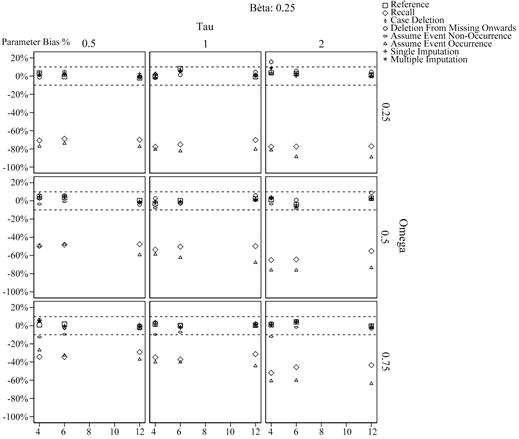
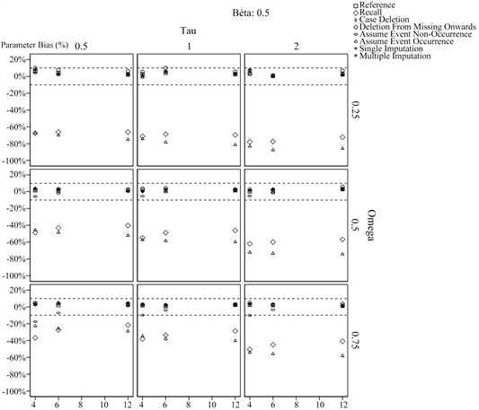
Figures 2-6 display the five criteria for evaluation as a function of the two parameters of the Weibull survival function (τ in the columns and ω in the rows) and the number of time periods (J on the horizontal axes) when the logit-effect size β = 0.5. Results for other values of β were very similar and can be found in the supplementary material. These results are further discussed later in this section. The reported results for the recall strategy in the figures are based on 40% probability of correctly remembering the missing event status, and other probabilities are evaluated later in this section.

3.3. Bias for β = 0.5

An analysis of variance showed that the main effect of strategy explains over 90 percent of the within-scenario variance (η² = 0.908), while only 7 percent of this variance was explained by the interaction effect between strategy and proportion of event occurrence in the control, i.e., ω (η² = 0.068). Proportion of event occurrence in the control, i.e., ω (η² = 0.616) and the shape parameter τ (η² = 0.283) explained about 90 percent of the variance at the between level. The number of time periods hardly explained any variance; neither did any of the interaction terms of which it was a part. The effects of the design factors are visualized in Figure 2. The two horizontal dashed lines represent a deviation of 10%. The difference between the strategies was largest when fewer subjects experienced the event (small ω) and/or when the probability of event occurrence rose to a peak at the end of the study (large τ).

Figure 2. Percentage Parameter bias. Results shown as a function of proportion event occurrence in the control condition ω (rows), shape parameter τ (columns) and number of periods J (horizontal line within each graph).

Figure 3. Average standard error. Results shown as a function of proportion event occurrence in the control condition ω (rows), shape parameter τ (columns) and number of periods J (horizontal line within each graph).

Figure 4. Percentage standard error bias. Results shown as a function of proportion event occurrence in the control condition ω (rows), shape parameter τ (columns) and number of periods J (horizontal line within each graph).

Figure 5. Coverage of confidence intervals. Results shown as a function of proportion event occurrence in the control condition ω (rows), shape parameter τ (columns) and number of periods J (horizontal line within each graph).

Figure 6. Empirical power. Results shown as a function of proportion event occurrence in the control condition ω (rows), shape parameter τ (columns) and number of periods J (horizontal line within each graph).

The percentage bias based on the analysis of complete data was slightly positive for all scenarios. It was equal to 2.4 on the average, with a maximum value of 6.4, which are acceptable values.

Three strategies showed a dramatically underestimated treatment effect. The first of these strategies with huge bias was the event-occurrence strategy. Biases ranged from −23% to −88% and the treatment effect was severely underestimated when fewer subjects experienced the event (smaller ω). This is obvious because the probability of an event within each time interval is small and assuming event occurrence in case of a missing value is a bad strategy. Furthermore, the underestimate became more severe when the probability of event occurrence increased over time (larger τ). In that case the probability of event occurrence is small in the first few time periods and it is likely subjects have a missing outcome before they experience the event.

The second strategy is the non-occurrence strategy, for which biases ranged from −17.4% to 4.8%. A large bias was observed for 4 or 6 time periods while it was less than 4% for 12 time periods. The bias was smaller than for the opposite strategy, which assumes event occurrence in case of a missing. This is obvious since, in our simulations, the probabilities of event occurrence in each time interval were rather small. In fact, they were hardly ever larger than 0.5, hence assuming event non-occurrence was better than assuming event occurrence in most scenarios. The bias became more severe when more subjects experienced the event (larger ω), which is obvious since the probability of event occurrence within a time interval is larger and assuming event non-occurrence in case of a missing event status is not a good strategy. Furthermore, the bias became more severe when the probability of event occurrence decreased over time (smaller τ). In such cases it is likely a time period with event occurrence precedes the time period with a missing event status, hence assuming event non-occurrence is not the best strategy.

The third strategy that shows a huge bias for the treatment effect relies on recall of the event status. Here, biases were always negative and ranged from −22% to −78%. The underestimate became more severe when fewer subjects experienced the event during the course of the study (smallerω) and/or when the probability of event occurrence was largest at the end of the study (larger τ).

We reason that this occurs because all three strategies have a given probability of providing the correct event status. For the strategy that assumes event occurrence, this probability is equal to the probability of the event occurring during the specific missing period. This in turn depends on ω and τ and will generally be low. For the strategy that assumed non-event occurrence, the probability of being correct is equal to one minus the probability of event occurrence. Therefore, where the former strategy performs worse for smaller ω and larger τ, inversely, the latter will perform worse for larger ω and smaller τ. The recall strategy has a probability of being correct of 40%. Since this probability is closer to the strategy that assumes event occurrence, the recall strategy will also perform worse for smaller ω and larger τ.

The remaining strategies (i.e., case deletion, period deletion, single imputation and multiple imputation) performed equally well with negligible biases for the treatment effect.

3.4. Average Standard Error for β = 0.5

Analysis of variance showed that the main effect of strategy explains almost 70 percent of the within-scenario variance (η² = 0.697). The interaction effect between strategy and proportion of event occurrence in the control, i.e., ω (η² = 0.186) and the interaction effect between strategy and the shape parameter τ (η² = 0.085) both explained a lower amount of the within-scenario variance (about 27 percent). The proportion of event occurrence in the control, i.e., ω (η² = 0.770) and the number of periods J (η² = 0.186) explained more than 90 percent of the variance between scenarios. The results are further visualized in Figure 3. As with bias, the difference between the strategies was largest when fewer subjects experienced the event (small ω) and/or when the probability of event occurrence was largest at the end of the study (large τ).

The largest average standard error was found for the strategy that deletes a subject’s data from the time period with missing event status onwards (i.e., period deletion strategy). For this strategy the average standard error was at most 112% higher than that of the analysis based on complete data. It increased when the probability of event occurrence became higher at the end of the study (increasing τ) when the number of time points J decreased and when fewer subjects experienced the event (decreasing ω). Multiple imputation also had marginally larger average standard errors than the analysis based on complete data, (in the most extreme case it was 27% higher). For this strategy the average standard error was larger with fewer time periods J.

For the strategy that relies on recall of event status and the strategy that assumes event occurrence, the average standard error was much smaller than the one based on complete data when ω = 0.25 or ω = 0.5. It was up to 33% and 39% smaller than the one based on complete data for the recall and the event occurrence strategy, respectively. The difference between the standard error of these strategies and the standard error of the complete data analysis increased when the number of time periods J increased. When ω = 0.75 the average standard error for these two strategies was mainly larger than the one based on complete data, and the relative difference increased when the number of time periods decreased and when the probability event occurrence was largest at the beginning of the trial.

For the other three strategies (i.e., case deletion, non-event occurrence and single imputation) the average standard error deviated by at most 15 percent from the one based on an analysis of complete data.

3.5. Standard Error Bias for β = 0.5

Most variation at the within-scenario level was explained by strategy (η² = 0.844), while the interaction between strategy and the number of periods explained a much lower amount of variation (η² = 0.110). In addition, the following effects explained more than six percent of variance at the between level: proportion of event occurrence in the control, i.e., ω (η² = 0.079), shape parameter τ (η² = 0.079), number of periods J (η² = 0.308), and the interaction τ* J (η² = 0.191). Figure 4 shows the standard error biases as a function of the design factors ω, τ and J. The two horizontal dashed lines represent a deviation of 5%.

The standard error bias based on complete data was always between −5 and +5 percent. This, however, was not the case for some of the strategies to deal with missing data. For all scenarios, single imputation and case deletion showed negative standard error biases which were as large as −23% and −22%, respectively. For both strategies the standard error biases decreased when the number of time periods increased. For multiple imputation, in contract, there were a few positive standard error biases over 10%, and there was no clear relation with the number of time periods. The standard error bias of the remaining methods was not noticeable.

3.6. Coverage Rate of Confidence Intervals for β = 0.5

Most of the variance at the within-scenario level was explained by strategy (η² = 0.744); a lower amount was explained by the interaction between strategy and the proportion event occurrence in the control condition ω (η² = 0.169). The highest amount of variance at the between level was explained by ω (η² = 0.734); the shape parameter τ explained a lower amount (η² = 0.203). Figure 5 shows an increasing difference between the strategies with increasing τ and decreasing ω.

All confidence intervals based on an analysis of complete data had a coverage rate within the range [0.936, 0.964]. The recall strategy as well as the event occurrence strategy showed a large degree of undercoverage of the confidence interval. For both strategies, all of the 27 confidence intervals had a coverage rate below 0.936. The degree of undercoverage increased with increasing τ, decreasing ω and increasing J. Given that the parameter bias for these two strategies was large, it was not surprising they resulted in a large degree of undercoverage.

Single imputation and case deletion strategies had also a lower degree of undercoverage. For both strategies, hardly any of the confidence intervals reached the nominal level of 95% (25 out of 27 confidence intervals had a coverage rate below 0.936). In contrast, multiple imputation performed better and most of the confidence intervals reached the nominal level 95%. We observed a slight over-coverage in some scenarios when the number of periods was small (10 out of 27 confidence intervals had a coverage rate above 0.964).

The last two strategies event non-occurrence and period deletion had an acceptable coverage rate as, respectively, 23 and 25 out of 27 confidence intervals were within the range [0.936, 0.964].

3.7. Power for β = 0.5

Almost all of the variance at the within-scenario level was explained by strategy (η² = 0.929). Design factors that explained more than 6 percent of the variance at the between level were the number of periodsJ (η² = 0.154) and the proportion of event occurrence in the control condition, i.e., ω (η² = 0.78). The effects of other design factors and interactions were less than medium size. Figure 6 shows that the difference between the power levels of the strategies increased when more subjects experienced the event (increasing ω). In general power increased with increasing number of time periods J and increasing proportion of subjects in the control who experienced the event (ω). In almost all scenarios the highest power was observed for an analysis based on complete data. Power was somewhat lower for single imputation and case deletion.

The lowest power levels were observed for the following strategies: recall, event occurrence and period deletion. For the first two strategies, the low power followed from the underestimate of the treatment effect; for the last strategy it followed from an overestimate of the standard error.

A smaller loss of power was observed for multiple imputation and the event non-occurrence strategy. For the former the loss of power was a result of an overestimate of the standard error, while, for the latter, it was a result of an underestimate of the treatment effect.

3.8. Main Findings for Other Values of β

The supplementary material shows mixed design analysis of variance results for other values of the logit effect sizeβ, with all η² > 0.06 highlighted in yellow, and figures similar to Figures 2-6.

A visual inspection of the graphs shows that the bias, average standard error and standard error bias were hardly affected by the treatment effect β. However, the coverage and power where somehow affected by different values of β. More specifically, the strategies provided higher coverage rates (closer to the nominal level 0.95) when β was small. Moreover, the larger the treatment effectβ was, the larger the differences between the coverage rates became. Furthermore, empirical power increased with increasing effect size (i.e., a larger value of β), which is obvious since larger effects have a higher probability to be detected by a statistical test. Also, the difference in power between the strategies increased with increasing effect size. In general, we can conclude that those strategies that did not perform well for a given criterion for evaluation for β = 0.5 also did not perform well for the same criterion and other values β.

The mixed design analysis of variance tables show that most variance at the within-scenario level was explained by strategy while the proportion of event occurrence in the control condition, i.e., ω explained in most cases the highest amount of variance at the between level.

3.9. The Effect of the Probability of Correctly Remembering Event Status in the Recall Strategy

The results for the recall strategy in Figures 2-6 were based on a 40% probability of correctly remembering the missing event status. Figure 7 presents results for this and two other probabilities as a function of the number of time periods J and for β = 0.5, ω = 0.5 and τ = 1. In general, better results were obtained when the probability of a correct recall increased.

The left panel at the top row shows that the treatment effect size was underestimated. Even when the correct recall probability was as high as 75%, the bias was at least 20%. An even larger bias was observed when this probability decreased. The bias decreased when the number of time periods increased. The right panel at the top shows the standard error decreased with increasing number of time periods. The standard error became smaller when the correct recall probability decreased, especially so when J = 6 or 12. The left panel in the middle row shows the standard error bias was less than 5% in all cases and there did not appear to be a relation with the probability of correctly remembering the even status. The right panel in the middle rows shows that in all cases the coverage of the confidence intervals was too low, even when the probability of correctly remembering the even status was as high as 75%. The panel in the lower row shows empirical power decreased when the correct recall probability decreased, and it increased with the number of time periods.

4. Empirical Example

The IMPACT study at the University of Massachusetts AIDS Unit, abbreviated to UIS, was a 5-year (1989-1994) collaborative research project comprised of two concurrent randomized trials of residential treatment for drug abuse. A group of residents was randomized to either a short or long residential treatment program. The purpose of the study was to compare treatment programs of different planned durations designed to reduce drug abuse and to prevent high-risk HIV behavior. Here, we use a subset of 629 participants of the UIS data [22] for a purely methodological exercise to illustrate the performance of various imputation strategies in handling missing event status in a survival endpoint analysis.

In the IMPACT study, the event of interest was defined as whether the participants relapsed to drugs or were lost to follow-up. The time to event was measured continuously (in days). We have therefore converted the time to event to discrete points in time in order to accommodate a discrete-time survival analysis. We initially assumed a study with a maximum observation time of 2 years (i.e., 730 days) where event occurrence was taken at the end of each quarter (i.e., whether the participants returned to drugs or lost to follow-up was recorded at each of 8 time periods). There were 5 participants who had a survival of more than 2 years and therefore their survival time was censored. In addition to the treatment indicator, the data set contained measurements recorded at baseline. These baseline variables, however, were not fully observed causing to remove 53 participants from the study. This leads to a total of 575 participants of which 289 participants were in the short treatment program and 286 in the long treatment program.

Figure 7. Results for the recall strategy. Results are shown for the various values of the probability to correctly remember the missing event status. Legend: □ = 25% probability, △ = 40% probability, ○ = 75% probability.

The original data did not have any missing values in the event status. Therefore, we created missing data artificially for the event status in the same manner as we did in our simulation study. More specifically, each participant had at most one missing value in the event status. For instance, if the second time point was set to missing for a particular participant, the event status was observed in the other time periods for that participant. This procedure resulted in approximately 40% of participants who had one missing value in the event status. For the remaining 60%, the missing came after event occurrence.

The incomplete data set was further imputed by different methods summarized in Table 1. The resulting completed data set was afterwards analyzed using the discrete-time survival model presented in Equation (5). The following baseline measurements were also included in the analysis model: age, Beck depression score, the number of prior drug treatments and race. For multiple imputation, we generated 100 completed datasets using the R package mice (version 3.3.0) and fitted the discrete-time survival model in Equation (5) to each imputed dataset. The estimates from multiply imputed datasets were then combined using Rubin’s rule to make a single estimate of the parameters. Table 2 gives point estimates of the treatment effect from the different strategies.

Table 2. Results for the empirical example for different strategies.

The first row of Table 2 shows the estimate of the treatment effect before introducing missing event status (i.e., complete data). It therefore can be considered as a benchmark for the strategies to deal with missing data. The case deletion method, where participants with missing event status are removed, showed a negatively biased estimate of the treatment effect while the same effect was positively biasedly estimated by the period deletion method. Both versions of the deletion methods had an increased standard error (due to a reduced sample size), which, in turn, resulted in a wider confidence interval for both methods (see rows 3 and 4 of Table 2).

The naive imputation methods including single imputation also resulted in a biased estimate of the treatment effect. In particular, the method that assumes the event had occurred had the worst performance (the estimate of the treatment effect was two times smaller than that of the complete data). The recall method, when each participant was asked to recall the event status of the previous period, also underestimated the treatment effect. Moreover, the standard error of these methods differed marginally compared to the standard error from the complete data.

Multiple imputation, as opposed to the other methods, showed a negligible bias in the estimate of the treatment effect (its estimate was −0.26 as compared to the estimated value of −0.25 from the complete data). However, its standard error was somewhat larger than that of the complete data, resulting in a slightly wider confidence interval. This is expected because multiple imputation always considers the uncertainty about which value to impute.

In sum, we can conclude that multiple imputation outperforms the other simple methods, and the findings from the empirical example are in line with what we have found in the simulation study.

5. Discussion

Missing data poses a particular problem in discrete-time survival analysis since subjects are only followed until event occurrence. If a subject’s event occurrence is unknown during intermittent time periods, it is unclear whether it needs to be measured at subsequent time periods. The goal of this study was to compare several strategies (Table 1), which can be used to manage this difficult problem, in order to facilitate future research on survival analysis. These strategies were evaluated using six criteria (convergence rate, parameter bias, average standard error, standard error bias, coverage rate of confidence intervals and empirical power) in a simulation study based on a Weibull survival function. A series of mixed design analyses of variance indicated that most of the within-variance was explained by strategy.

Table 3 shows a summary of results for each of the criteria for evaluation. The strategies assuming event occurrence and event non-occurrence together with the recall strategy had the worst performance because of a substantial parameter bias and a sharp decrease in coverage rate. In particular, the event occurrence strategy and the recall strategy failed in four out of five criteria. Period deletion showed a huge increase of standard error (as compared to complete data) resulted from removing a large amount of information, which, in turn, caused an unacceptable loss of power. Case deletion also had a negative standard error bias followed by an undercoverage rate. The latter can be particularly problematic because it inflates the type I error. Single imputation suffered from the undercoverage issue too as a result of a negative standard error bias. This is expected because single imputation is known to underestimate the standard error. Multiple imputation, in contrast, showed a reasonable performance, with only a negligible, positive standard error bias. Comparing to single imputation, the empirical standard error for multiple imputation is larger, since the latter takes two sources of variation (both within and between imputation) into account while the former only has the within variance. This was also shown in our results, as multiple imputation overestimated the standard error. This overestimation of the standard error leads to a gradual decrease in power with multiple imputation, which was also shown in our results.

Table 3. Summary of conclusions based on our simulation results.

This paper was restricted in a three ways. Firstly, although the period in which a subject might have a missing outcome is generated randomly (from p = 1 to 12), the subject could only have a missing value if that subject was still in the study. Therefore, the process, which created missing data implicitly depended on whether the subject had been observed until that period. Consequently, the missing data mechanism can be classified as missing at random (MAR) instead of missing completely at random (MCAR). Future research could focus on whether these results also hold when the data are MCAR, or even under missing not at random (MNAR) when the missingness is nonignorable. Secondly, subjects were limited to a maximum of one missing period. However, in real life, subjects are likely to miss more than just one period. Although more missingness will likely worsen the results, it is unlikely to affect which strategy is best suited for the management of missing data. A third limitation was that only a Weibull survival function was used. Although the Weibull survival function allows for the hazard to increase or decrease over time, it does not allow the hazard to have one or more peaks or troughs throughout the study. However, given the variety of scenarios in which the strategies were tested, we do not believe another function would have yielded different results. Similarly, we do not expect other results for other values of the sample size, treatment effect size and number of time periods.

A recent, similar study by Jolani and Safarkhani [23] also investigated strategies to manage missing data in survival analyses. However, that study focused on missing data in the baseline covariates. Baseline covariates are often used in statistical models in experimental studies to take the heterogeneity between individuals into account, which increases the power of these models. However, often the baseline covariates have some missing data. Strategies that handle those missing data were studied and it was found that single and multiple imputation methods outperformed other strategies, among which was complete case analysis.

6. Conclusion

In the present study, as opposed to Jolani and Safarkhani [23], it was found that single imputation could underestimate the standard error, which leads to an overstatement of significant effects (type I error) and to an undercoverage of the confidence interval, while multiple imputation performed satisfactorily. It would be interesting to further evaluate and compare different strategies when both the event occurrence and baseline covariates have missing data. Also, future work could focus on more extensive simulation studies that overcome the three restrictions of the simulation study in this paper: it should focus on MCAR or even MNAR missing data structures, it should focus on more than one missing per person and it should focus on survival functions other than the Weibull function.

Mixed Design ANOVA Analyses on Results of Simulation Study

Supplementary material to:

An evaluation of strategies to deal with missing outcomes in discrete-time event history analysis.

Bias

Bias for beta = 0.25

Note. Type III Sum of Squares. ^aMauchly’s test of sphericity indicates that the assumption of sphericity is violated (p < 0.05).

Note. Type III Sum of Squares.

Bias for beta = 0.5

Note. Type III Sum of Squares. ^aMauchly’s test of sphericity indicates that the assumption of sphericity is violated (p < 0.05).

Note. Type III Sum of Squares.

Bias for beta = 1

Note. Type III Sum of Squares. ^aMauchly’s test of sphericity indicates that the assumption of sphericity is violated (p < 0.05).

Note. Type III Sum of Squares.

Average standard error

Average standard error for beta = 0.25

Note. Type III Sum of Squares. ^aMauchly’s test of sphericity indicates that the assumption of sphericity is violated (p < 0.05).

Note. Type III Sum of Squares.

Average standard error for beta = 0.5

Note. Type III Sum of Squares. ^aMauchly’s test of sphericity indicates that the assumption of sphericity is violated (p < 0.05).

Note. Type III Sum of Squares.

Average standard error for beta = 1

Note. Type III Sum of Squares.

Note. Type III Sum of Squares.

Standard error bias

Standard error bias for beta = 0.25

Note. Type III Sum of Squares. ^aMauchly’s test of sphericity indicates that the assumption of sphericity is violated (p < 0.05).

Note. Type III Sum of Squares.

Standard error bias for beta = 0.5

Note. Type III Sum of Squares. ^aMauchly’s test of sphericity indicates that the assumption of sphericity is violated (p < 0.05).

Note. Type III Sum of Squares.

Standard error bias for beta = 1

Note. Type III Sum of Squares. ^aMauchly’s test of sphericity indicates that the assumption of sphericity is violated (p < 0.05).

Note. Type III Sum of Squares.

Coverage

Coverage for beta = 0.25

Note. Type III Sum of Squares.

Note. Type III Sum of Squares.

Coverage for beta = 0.5

Note. Type III Sum of Squares. ^aMauchly’s test of sphericity indicates that the assumption of sphericity is violated (p < 0.05).

Note. Type III Sum of Squares

Coverage for beta = 1

Note. Type III Sum of Squares. ^aMauchly’s test of sphericity indicates that the assumption of sphericity is violated (p < 0.05).

Note. Type III Sum of Squares.

Power

Power for beta = 0.25

Note. Type III Sum of Squares.

Note. Type III Sum of Squares.

Power for beta = 0.5

Note. Type III Sum of Squares.

Note. Type III Sum of Squares.

Power for beta = 1

Note. Type III Sum of Squares. ^a Mauchly’s test of sphericity indicates that the assumption of sphericity is violated (p < 0.05).

Note. Type III Sum of Squares.

Conflicts of Interest

The authors declare no conflicts of interest.

References

[1]	Cox, D. (1972) Regression Models and Life Tables. Journal of the Royal Statistical Society Series B, 34, 187-220. https://doi.org/10.1111/j.2517-6161.1972.tb00899.x
[2]	Moerbeek, M. and Schormans, J. (2015) The Effect of Discretizing Survival Times in Randomized Controlled Trials. Methodology, 11, 55-64. https://doi.org/10.1027/1614-2241/a000091
[3]	Singer, J.D. and Willett, J.B. (2003) Applied Longitudinal Data Analysis: Modeling Change and Event Occurrence. Oxford University Press, Oxford.
[4]	Singer, J.D. and Willett, J.B. (1993) It’s About Time: Using Discrete-Time Survival Analysis to Study Duration and the Timing of Events. Journal of Educational and Behavioral Statistics, 18, 155-195. https://doi.org/10.3102/10769986018002155
[5]	Hox, J., Moerbeek, M. and Van de Schoot, R. (2018) Multilevel Analysis. Techniques and Applications. 3rd Edition, Routledge, Boca Raton. https://doi.org/10.4324/9781315650982
[6]	Tan, F., Jolani, S. and Verbeek, H. (2018). Guidelines for Multiple Imputations in Repeated Measurements with Time-Dependent Covariates: A Case Study. Journal of Clinical Epidemiology, 102, 107-114. https://doi.org/10.1016/j.jclinepi.2018.06.006
[7]	Schafer, J.L. and Graham, J.W. (2002) Missing Data: Our View of the State of the Art. Psychological Methods, 7, 147-177. https://doi.org/10.1037/1082-989X.7.2.147
[8]	Rubin, D. (1976) Inference and Missing Data. Biometrika, 63, 581-592. https://doi.org/10.1093/biomet/63.3.581
[9]	Little, R. and Rubin, D. (2002) Statistical Analysis with Missing Data. Wiley, New York. https://doi.org/10.1002/9781119013563
[10]	Hedeker, D. and Gibbons, R.D. (2006) Longitudinal Data Analysis. Wiley, Hoboken.
[11]	Duncan, T.E., Duncan. S.C. and Strycker, L.A. (2006) An Introduction to Latent Variable Growth Curve Modeling. 2nd Edition, Erlbaum, Mahwah.
[12]	Bollen, K. and Curran, P. (2006) Latent Curve Models. A Structural Equation Perspective. Wiley, Hoboken. https://doi.org/10.1002/0471746096
[13]	Little, T. (2013) Longitudinal Structural Equation Modeling. Guilford Press, New York.
[14]	Newsom, J. (2015) Longitudinal Structural Equation Modeling. Routledge, New York. https://doi.org/10.4324/9781315871318
[15]	Treiman, D.J. (2008) Quantative Data Analysis. Jossey-Bass, San Francisco.
[16]	Van Buuren, S. (2018) Flexible Imputation of Missing Data. 2nd Edition, CRC Press, Boca Raton. https://doi.org/10.1201/9780429492259
[17]	R Core Team (2018) R: A Language and Environment for Statistical Computing. R Foundation for Statistical Computing, Vienna.
[18]	Van Buuren, S., Groothuis-Oudshoorn, K., Robitzsch, A., Vink, G., Doove, L. and Jolani, S. (2015) Package “Mice”, Computer Software. https://cran.r-project.org/web/packages/mice/index.html
[19]	Muthén, L.K. and Muthén, B.O. (2002) How to Use a Monte Carlo Study to Decide on Sample Size and Determine Power. Structural Equation Modeling, 9, 599-620. https://doi.org/10.1207/S15328007SEM0904_8
[20]	Cohen, J. (1988) Statistical Power Analysis for the Behavioral Sciences. 2nd Edition, Erlbaum, Hillsdale.
[21]	IBM Corp. (2016) IBM SPSS Statistics for Windows, Version 24.0. IBM Corp., Armonk.
[22]	Hosmer, D.W., Lemeshow, S. and May, S. (2008) Applied Survival Analysis. Regression Modeling of Time-to-Event Data. 2nd Edition, Wiley, Hoboken. https://doi.org/10.1002/9780470258019
[23]	Jolani, S. and Safarkhani, M. (2017) The Effect of Partly Missing Covariates on Statistical Power in Randomized Controlled Trials with Discrete-Time Survival Endpoints. Methodology, 13, 41-60. https://doi.org/10.1027/1614-2241/a000121