A Series Solution Approach to the Circular Restricted Gravitational Three-Body Dynamical Problem

Maha Hamed Alghamdi, Aisha Abdu Alshaery^*

Department of Mathematics, Faculty of Science, University of Jeddah, Jeddah, KSA.

DOI: 10.4236/jamp.2020.812200                

Abstract

The present manuscript examines the circular restricted gravitational three-body problem (CRGTBP) by the introduction of a new approach through the power series method. In addition, certain computational algorithms with the aid of Mathematica software are specifically designed for the problem. The algorithms or rather mathematical modules are established to determine the velocity and position of the third body’s motion. In fact, the modules led to accurate results and thus proved the new approach to be efficient.

Keywords

n-Body Problems, Restricted Gravitational Problems, Power Series Method, Series Solution Approach

1. Introduction

The circular restricted gravitational three-body problem (CRGTBP) is a special case of the gravitational three-body problem which is one of the most important n-body problems. The CRGTBP consists of three bodies; the two bodies of them (which are referred to as the primaries or the primary and the secondary) are moving in a circular orbit about their common mass’s center under the influence of their mutual gravitation and the third body is infinitesimal mass moving under the gravitational significance of the two masses where its mass cannot influence the two masses. Furthermore, the third body has a common plane of movement as defined by both the primary and secondary [1] - [6]. The problem is tackled by studying the motion of the third body assuming full knowledge of the primary and the secondary with regards to their motions [1] [2] [7] [8].

Many physicists and mathematicians have used the method of power series to solve a variety of unsolvable differential equations. The method has been used significantly to solve the celestial mechanic problems as better exactness of inspectional data is required for relatively optimal solutions to the bodies’ dynamical equations of motion. Numerous scientists have used this method including Saad et al. [9] that used it to get recurrent algorithm for comets under non-gravitational motion. Rabe [10] used a new computational and iteration method to determine a series of periodic Trojan orbits in the restricted problem of three bodies. Deprit and Price [11] used the numerical methods to compute characteristic exponents in the planar restricted problem of three bodies. Sharaf et al. [12] found symbolic solution of the three-dimensional restricted three-body problem and applied it for any given set of initial values.

However, we aim in this paper to employ an approach based on the power series to establish an algorithm or mathematical module using Mathematica to tackle this important problem of circular restricted gravitational dynamical problem. More specifically, we determine the components of the velocity and position vectors of the third body with regard to the CRGTBP.

2. Dynamical Equations of Motion of CRGTBP

The dynamical equations of motion for the CRGTBP are given by the following coupled first-order system as follows [12]

$\begin{array}{l}\stackrel{\dot{}}{x}=u,\\ \stackrel{\dot{}}{y}=v,\\ \stackrel{\dot{}}{z}=w,\\ \stackrel{\dot{}}{u}=\left(\mu -1\right)\left(\frac{x-\mu }{r_1^3}\right)-\mu \left(\frac{x+1-\mu }{r_2^3}\right)+x+2v,\\ \stackrel{\dot{}}{v}=\left(\mu -1\right)\left(\frac{y}{r_1^3}\right)-\mu \left(\frac{y}{r_2^3}\right)+y-2u,\\ \stackrel{\dot{}}{w}=\left(\mu -1\right)\left(\frac{z}{r_1^3}\right)-\mu \left(\frac{z}{r_2^3}\right),\end{array}$ (1)

where $\left(\mu \mathrm{,0,0}\right)$, $\left(-\left(1-\mu \right)\mathrm{,0,0}\right)$ and $\left(x\mathrm{,}y\mathrm{,}z\right)$, are the coordinates of the primary, the secondary and the third body, respectively. More, $\mu$ is the primary’s mass, $1-\mu$ is the secondary’s mass ( $\mu$ is larger than $1-\mu$, where $\mu \in \left[\mathrm{0,}\frac{1}{2}\right]$ ). $G=1$ is the unit of the force of a gravitational constant; with $r_1$ denoting the distance of the primary and $r_2$ that of the secondary both to the third body [1] [2] [6] [13] given by

$\begin{array}{l}{r}_1=\sqrt{{\left(x-\mu \right)}^2+y^2+z^2},\\ r_2=\sqrt{{\left(x+1-\mu \right)}^2+y^2+z^2}.\end{array}$ (2)

Using Broucke’s method [14], the following system of first-order differential equations [12] is thus obtained

$\begin{array}{l}\stackrel{\dot{}}{x}=u,\\ \stackrel{\dot{}}{y}=v,\\ \stackrel{\dot{}}{z}=w,\\ \stackrel{\dot{}}{u}=\left(\mu -1\right)\left(x-\mu \right)s_1-\mu \left(x-\mu +1\right)s_2+x+2v,\\ \stackrel{\dot{}}{v}=\left(\mu -1\right)s_1-\mu y{s}_2+y-2u,\end{array}$

$\begin{array}{l}\stackrel{\dot{}}{w}=\left(\mu -1\right)z{s}_1-\mu z{s}_2,\\ r_1{\stackrel{\dot{}}{r}}_1=\left(x-\mu \right)\stackrel{\dot{}}{x}+y\stackrel{\dot{}}{y}+z\stackrel{\dot{}}{z},\\ r_2{\stackrel{\dot{}}{r}}_2=\left(x-\mu +1\right)\stackrel{\dot{}}{x}+y\stackrel{\dot{}}{y}+z\stackrel{\dot{}}{z},\\ {\stackrel{\dot{}}{s}}_1{r}_1=-3s_1{\stackrel{\dot{}}{r}}_1,\\ {\stackrel{\dot{}}{s}}_2{r}_2=-3s_2{\stackrel{\dot{}}{r}}_2.\end{array}$ (3)

3. Solution by Power Series

The equations given in (3) are unsolvable analytically. Therefore, these equations are solved in this section using the power series method and their analytical solutions are given in terms of recurrence relations of the coefficients posed by the variables.

Thus, with the use of the method of power series, the motion’s variables are as follows [12] [14]

$x={\displaystyle \underset{n=1}{\overset{\infty }{\sum }}}{X}_n{t}^{n-1},y={\displaystyle \underset{n=1}{\overset{\infty }{\sum }}}{Y}_n{t}^{n-1},z={\displaystyle \underset{n=1}{\overset{\infty }{\sum }}}{Z}_n{t}^{n-1},$

$u={\displaystyle \underset{n=1}{\overset{\infty }{\sum }}}{U}_n{t}^{n-1},v={\displaystyle \underset{n=1}{\overset{\infty }{\sum }}}{V}_n{t}^{n-1},w={\displaystyle \underset{n=1}{\overset{\infty }{\sum }}}{W}_n{t}^{n-1},$

$r_1={\displaystyle \underset{n=1}{\overset{\infty }{\sum }}}{R}_{1n}{t}^{n-1},r_2={\displaystyle \underset{n=1}{\overset{\infty }{\sum }}}{R}_{2n}{t}^{n-1},$

$s_1={\displaystyle \underset{n=1}{\overset{\infty }{\sum }}}{S}_{1n}{t}^{n-1},s_2={\displaystyle \underset{n=1}{\overset{\infty }{\sum }}}{S}_{2n}{t}^{n-1}.$

In these power series, the first coefficients are given by the known initial values of $\left(x_0\mathrm{,}{y}_0\mathrm{,}{z}_0\mathrm{,}{u}_0\mathrm{,}{v}_0\mathrm{,}{w}_0\right)$ as follows [12]

$X_1=x_0,Y_1=y_0,Z_1=z_0,$

$U_1=u_0={\stackrel{\dot{}}{x}}_0,V_1=v_0={\stackrel{\dot{}}{y}}_0,W_1=w_0={\stackrel{\dot{}}{z}}_0,$

$R_{11}=\sqrt{{\left(x_0-\mu \right)}^2+y_0^2+z_0^2},$

$R_{21}=\sqrt{{\left(x_0+1-\mu \right)}^2+y_0^2+z_0^2},$

$S_{11}={\left(R_{11}\right)}^{-3},S_{21}={\left(R_{21}\right)}^{-3}.$

The following recurrence relations for the remaining coefficients are found using power series [12]

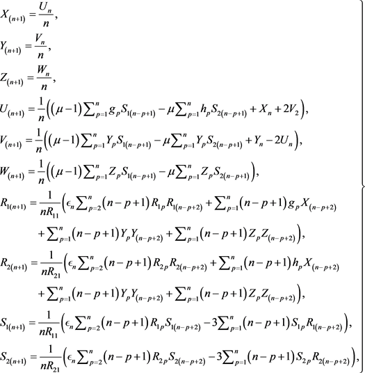(4)

where

$g_n=(\begin{array}{ll}{X}_1-\mu ,\hfill & \text{if}n=1,\hfill \\ X_n,\hfill & \text{if}n\ge 2,\hfill \end{array}$

$h_n=(\begin{array}{ll}{X}_1+1-\mu ,\hfill & \text{if}n=1,\hfill \\ X_n,\hfill & \text{if}n\ge 2,\hfill \end{array}$

${ϵ}_n=(\begin{array}{cc}\mathrm{0,}& \text{if}n=\mathrm{1,}\\ -\mathrm{1,}& \text{if}n\ge 2.\end{array}$

4. Algorithm for CRGTBP

* Purpose

To generate the components of position and velocity for the third body at any time.

* Input

$x_0$, $y_0$, $z_0$, $u_0$, $v_0$, $w_0$, $\mu$, t and NN.

* Output

The components of position and velocity for the third body at any time.

* Module list.

$\text{Module}[\left\{\right\}\mathrm{,}X\left(1\right)=\text{x0}\mathrm{<mo>\; ;\; </mo>}Y\left(1\right)=\text{y0}\mathrm{<mo>\; ;\; </mo>}Z\left(1\right)=\text{z0}\mathrm{<mo>\; ;\; </mo>}$

$U\left(1\right)=\text{u0}\mathrm{<mo>\; ;\; </mo>}V\left(1\right)=\text{v0}\mathrm{<mo>\; ;\; </mo>}W\left(1\right)=\text{w0}\mathrm{<mo>\; ;\; </mo>}$

$R\left(\mathrm{1,1}\right)=\sqrt{{\text{y0}}^2+{\text{z0}}^2+{\left(\text{x0}-\mu \right)}^2}\mathrm{<mo>\; ;\; </mo>}$

$R\left(\mathrm{2,1}\right)=\sqrt{{\text{y0}}^2+{\text{z0}}^2+{\left(\text{x0}-\mu +1\right)}^2}\mathrm{<mo>\; ;\; </mo>}k=-\mathrm{3\; <mo>\; ;\; </mo>}$

$S\left(\mathrm{1,1}\right)=R{\left(\mathrm{1,1}\right)}^k\mathrm{<mo>\; ;\; </mo>}$

$S\left(\mathrm{2,1}\right)=R{\left(\mathrm{2,1}\right)}^k\mathrm{<mo>\; ;\; </mo>}$

$g\left(\text{n\_}\right):=X\left(1\right)-\mu \text{/};n=\mathrm{1\; <mo>\; ;\; </mo>}$

$g\left(\text{n\_}\right):=X\left(n\right)/;n\ge 2;$

$h\mathrm{<mo\; stretchy="false">\; (\; </mo>}\left(\text{n\_}\right):=-\mu +X\left(1\right)+1/;n=1;$

$h\left(\text{n\_}\right):=X\left(n\right)/;n\ge 2;$

$ϵ\left(\text{n\_}\right):=0\text{/};n=\mathrm{1\; <mo>\; ;\; </mo>}$

$ϵ\left(\text{n\_}\right):=-1\text{/};n\ge \mathrm{2\; <mo>\; ;\; </mo>}$

$\text{Do}[\{X\left(n+1\right)=\frac{U\left(n\right)}{n}\mathrm{,}x={\displaystyle \underset{n=1}{\overset{\text{NN}}{\sum }}}X\left(n\right)t^{n-1}\mathrm{,}$

$Y\left(n+1\right)=\frac{V\left(n\right)}{n}\mathrm{,}y={\displaystyle \underset{n=1}{\overset{\text{NN}}{\sum }}}Y\left(n\right)t^{n-1}\mathrm{,}$

$Z\left(n+1\right)=\frac{W\left(n\right)}{n}\mathrm{,}z={\displaystyle \underset{n=1}{\overset{\text{NN}}{\sum }}}Z\left(n\right)t^{n-1}\mathrm{,}$

$\text{Q1}=-\left(1-\mu \right){\displaystyle \underset{p\mathrm{<mo>\; =\; </mo>1}}{\overset{n}{\sum }}}g\left(p\right)S\left(\mathrm{1,}n-p+1\right)$

$-\mu {\displaystyle \underset{p=1}{\overset{n}{\sum }}}h\left(p\right)S\left(\mathrm{2,}n-p+1\right)+2V\left(n\right)+X\left(n\right)\mathrm{,}$

$U\left(n+1\right)=\frac{\text{Q1}}{n}\mathrm{,}u={\displaystyle \underset{n=1}{\overset{\text{NN}}{\sum }}}U\left(n\right)t^{n-1}\mathrm{,}$

$\text{Q2}=-\left(1-\mu \right){\displaystyle \underset{p=1}{\overset{n}{\sum }}}Y\left(p\right)S\left(\mathrm{1,}n-p+1\right)$

$-\mu {\displaystyle \underset{p=1}{\overset{n}{\sum }}}Y\left(p\right)S\left(\mathrm{2,}n-p+1\right)-2U\left(n\right)+Y\left(n\right)\mathrm{,}$

$V\left(n+1\right)=\frac{\text{Q2}}{n}\mathrm{,}v={\displaystyle \underset{n=1}{\overset{\text{NN}}{\sum }}}V\left(n\right)t^{n-1}\mathrm{,}$

$\text{Q7}=-\left(1-\mu \right){\displaystyle \underset{p=1}{\overset{n}{\sum }}}Z\left(p\right)S\left(\mathrm{1,}n-p+1\right)$

$-\mu {\displaystyle \underset{p=1}{\overset{n}{\sum }}}Z\left(p\right)S\left(\mathrm{2,}n-p+1\right)\mathrm{,}$

$W\left(n+1\right)=\frac{\text{Q7}}{n}\mathrm{,}w={\displaystyle \underset{n=1}{\overset{\text{NN}}{\sum }}}W\left(n\right)t^{n-1}\mathrm{,}$

$\text{Q3}={\displaystyle \underset{p=1}{\overset{n}{\sum }}}\left(n-p+1\right)g\left(p\right)X\left(n-p+2\right)$

$+{\displaystyle \underset{p=1}{\overset{n}{\sum }}}\left(n-p+1\right)Y\left(p\right)Y\left(n-p+2\right)$

$+{\displaystyle \underset{p=1}{\overset{n}{\sum }}}\left(n-p+1\right)Z\left(p\right)Z\left(n-p+2\right)$

$+\left({\displaystyle \underset{p=2}{\overset{n}{\sum }}}\left(n-p+1\right)R\left(\mathrm{1,}p\right)R\left(\mathrm{1,}n-p+2\right)\right)ϵ\left(n\right)\mathrm{,}$

$R\left(\mathrm{1,}n+1\right)=\frac{\text{Q3}}{nR\left(\mathrm{1,1}\right)}\mathrm{,}\text{Q4}={\displaystyle \underset{p=1}{\overset{n}{\sum }}}\left(n-p+1\right)h\left(p\right)X\left(n-p+2\right)$

$+{\displaystyle \underset{p=1}{\overset{n}{\sum }}}\left(n-p+1\right)Y\left(p\right)Y\left(n-p+2\right)$

$+{\displaystyle \underset{p=1}{\overset{n}{\sum }}}\left(n-p+1\right)Z\left(p\right)Z\left(n-p+2\right)$

$+\left({\displaystyle \underset{p=2}{\overset{n}{\sum }}}\left(n-p+1\right)R\left(\mathrm{2,}p\right)R\left(\mathrm{2,}n-p+2\right)\right)ϵ\left(n\right)\mathrm{,}$

$R\left(\mathrm{2,}n+1\right)=\frac{\text{Q4}}{nR\left(\mathrm{2,1}\right)}\mathrm{,}$

$\text{Q5}=ϵ\left(n\right){\displaystyle \underset{p=2}{\overset{n}{\sum }}}\left(n-p+1\right)R\left(\mathrm{1,}p\right)S\left(\mathrm{1,}n-p+2\right)$

$-3{\displaystyle \underset{p=1}{\overset{n}{\sum }}}\left(n-p+1\right)S\left(\mathrm{1,}p\right)R\left(\mathrm{1,}n-p+2\right)\mathrm{,}$

$S\left(\mathrm{1,}n+1\right)=\frac{\text{Q5}}{nR\left(\mathrm{1,1}\right)}\mathrm{,}$

$\text{Q6}=ϵ\left(n\right){\displaystyle \underset{p=2}{\overset{n}{\sum }}}\left(n-p+1\right)R\left(\mathrm{2,}p\right)S\left(\mathrm{2,}n-p+2\right)$

$-3{\displaystyle \underset{p=1}{\overset{n}{\sum }}}\left(n-p+1\right)S\left(\mathrm{2,}p\right)R\left(\mathrm{2,}n-p+2\right)\mathrm{,}$

$S\left(\mathrm{2,}n+1\right)=\frac{\text{Q6}}{nR\left(\mathrm{2,1}\right)}\}\mathrm{,}\left\{n\mathrm{,1,}\text{NN}\right\}]]$

5. Application for CRGTBP

For a numerical example of CRGTBP algorithm, the initial values of components for the position and velocity vectors are considered to be

$x_0=-0.153910449,y_0=0.886499068,z_0=0.384340387,$

$u_0=-0.00000000017268248,v_0=-0.0000000002545393,$

$w_0=-0.0000000001103033,\mu =\mathrm{0.0121505816.}$

Then, we get the final value components for the position and velocity vectors as given in Figures 1-12.

It is remarkable to mention here that the accuracy is increased with an increase in the number of terms of the power series, but after NN = 50, the accuracy is fixed. So, we aren’t needed to the more of terms of the power series.

Figure 1. Comparing the exact and approximate values for x when NN = 10.

Figure 2. Comparing the exact and approximate values for y when NN = 10.

Figure 3. Comparing the exact and approximate values for z when NN = 10.

Figure 4. Comparing the exact and approximate values for u when NN = 10.

Figure 5. Comparing the exact and approximate values for v when NN = 10.

Figure 6. Comparing the exact and approximate values for w when NN = 10.

Figure 7. Comparing the exact and approximate values for x when NN = 50.

Figure 8. Comparing the exact and approximate values for y when NN = 50.

Figure 9. Comparing the exact and approximate values for z when NN = 50.

Figure 10. Comparing the exact and approximate values for u when NN = 50.

Figure 11. Comparing the exact and approximate values for v when NN = 50.

Figure 12. Comparing the exact and approximate values for w when NN = 50.

6. Conclusion

In conclusion, the analytical solutions to the circular restricted gravitational three-body problem (CRGTBP) are determined via the application of the power series method. Also, a module or algorithm is specifically designed and implemented via the help of Mathematica software to find the components of the velocity and position vectors for the third body. Finally, the proposed methodology via the devised module has worked accurately and resulted in reliable results as shown.

Conflicts of Interest

The authors declare no conflicts of interest regarding the publication of this paper.

References

[1]	Roy, A.E. (2004) Orbital Motion. CRC Press, Boca Raton, Florida.
[2]	Frnka, R. (2010) The Circular Restricted Three-Body Problem. http://jan.ucc.nau.edu/~ns46/student/2010/Frnka_2010.pdf
[3]	Musielak, Z. and Quarles, B. (2017) Three Body Dynamics and Its Applications to Exoplanets. Springer, Cham. https://doi.org/10.1007/978-3-319-58226-9
[4]	Sharaf, M.A. and Alshaery, A.A. (2012) Restricted Three-Body Problem in Different Coordinate Systems. Applied Mathematics, 3, 949-953. https://doi.org/10.4236/am.2012.39142
[5]	Szebehely, V. (1967) Theory of Orbits: The Restricted Problem of Three Bodies. Academic Press Inc., New York. https://doi.org/10.1016/B978-0-12-395732-0.50007-6
[6]	Worthington, J. (2012) A Study of the Planar Circular Restricted Three Body Problem and the Vanishing Twist. Tese de Doutorado, University of Sydney, Sydney.
[7]	Barrow-Green, J. (1997) Poincaré and the Three Body Problem. American Mathematical Society, Providence, Rhode Island.
[8]	Heggie, D.C. (2005) The Classical Gravitational N-Body Problem. arXiv preprint astro-ph/0503600 https://doi.org/10.1016/B0-12-512666-2/00003-1
[9]	Saad, A.S., Banaszkiewicz, M. and Sitarski, G. (2008) A New Algorithm of the Recurrent Power Series Method for the Non-Gravitational Motion of Comets. Applied Mathematics and Computation, 197, 874-879. https://doi.org/10.1016/j.amc.2007.08.020
[10]	Rabe. E. (1961) Determination and Survey of Periodic Trojan Orbits in the Restricted Problem of Three Bodies. Astronomical Journal, 66, 500-513. https://doi.org/10.1086/108451
[11]	Deprit, A. and Price, J.F. (1965) The Computation of Characteristic Exponents in the Planar Restricted Problem of Three Bodies, (No. MN-415). Boeing Scientific Research Labs Seattle WA Mathematics Research Lab. https://doi.org/10.21236/AD0622985
[12]	Sharaf, M.A., Ghoneim, R. and Alshaery, A.A. (2011) Symbolic Solution of the Three Dimensional Restricted Three-Body Problem. Contributions of the Astronomical Observatory Skalnaté Pleso, 41, 1-12.
[13]	Valtonen, M. and Karttunen, H. (2006) The Three-Body Problem. Cambridge University Press, Cambridge. https://doi.org/10.1017/CBO9780511616006
[14]	Broucke, R. (1971) Solution of the N-Body Problem with Recurrent Power Series. Celestial Mechanics, 4, 110-115. https://doi.org/10.1007/BF01230326