Group Geometric Algebra and the Standard Model

Carl Brannen​

Retired, Pullman, WA, USA.

DOI: 10.4236/jmp.2020.118075                

Abstract

We show how to generalize the Weyl equation to include the Standard Model fermions and a dark matter fermion. The 2 × 2 complex matrices are a matrix ring R. A finite group G can be used to define a group algebra G[R] which is a generalization of the ring. For a group of size N, this defines N Weyl equations coupled by the group operation. We use the group character table to uncouple the equations by diagonalizing the group algebra. Using the full octahedral point symmetry group for G, our uncoupled Weyl equations have the symmetry of the Standard Model fermions plus a dark matter particle. We describe the symmetry properties of dark matter.

Keywords

Weyl Equation, Dark Matter, Standard Model

1. Introduction

We will write the Weyl equation [1] for a single massless fermion as

${\sigma }^{\mu }{\partial }_{\mu }\psi =I_2\frac{\partial \psi }{\partial t}\pm {\sigma }_x\frac{\partial \psi }{\partial x}\pm {\sigma }_y\frac{\partial \psi }{\partial y}\pm {\sigma }_z\frac{\partial \psi }{\partial z}=0,$ (1)

where $I_2$ is the 2 × 2 unit matrix, the ${\sigma }_j$ is the Pauli spin matrices. The plus signs are for the left handed Standard Model fermions and the minus signs are for the right handed fermions. In the above, the Pauli algebra has a basis of four 2 × 2 complex matrices $\left\{{\sigma }^{\mu }\right\}=\left\{{\sigma }_t,{\sigma }_x,{\sigma }_y,{\sigma }_z\right\}=\left\{I_2,{\sigma }_x,{\sigma }_y,{\sigma }_z\right\}$ where each of the four ${\sigma }^{\mu }$ has two nonzero complex elements. The wave function $\psi$ is a 1 × 2 vector so the Weyl equation consists of two coupled differential equations with four terms in each. We will generalize the ${\sigma }^{\mu }$ to ${\sigma }^{\mu g}$ so that they depend on a group element g. There will now be 4N different ${\sigma }^{\mu g}$ where N is the number of elements in the finite group G. These matrices are still linearly independent in the sense that

${\Sigma }_{\mu ,g}{a}_{\mu g}{\sigma }^{\mu g}=0$ (2)

implies that the 4N complex constants $a_{\mu g}$ are all zero.

Changing the signs of the Pauli spin matrices, as seen above in the left and right handed Weyl equations, can be thought of as a symmetry operation. The symmetry group has two elements, it is the point group symmetry that Hestenes and Holt [2] call $\overline{22}$. We will label the point group symmetries we use with their notation and to avoid confusion with numerals will prepend them with “Geo” as in $\text{Geo}\overline{22}$. The groups explored in this paper are the full octahedral group Geo43, some of its subgroups and a tripled Geo43 with $48\times 3=144$ elements we will call 3Geo43. An element of Geo43 or its subgroups can be described by its effect on the Pauli spin matrices. In general, the three matrices can be permuted and can be independently negated. Together, these give the $\mathrm{3\; <mo>\; !\; </mo>}\times 2^3=48$ elements of Geo43.

The finite point group $\text{Geo}\overline{22}$ is a good example to make clear how we are generalizing the Weyl equation. First, to make our notation concise and descriptive, let’s define the two elements of the group as $\text{Geo}\overline{22}=\left\{(+),(-)\right\}$ so that the multiplication rules are $(+)(+)=(+)$, $(+)(-)=(-)$, $(-)(+)=(-)$ and $(-)(-)=(+)$. Then the eight generalizations of the four Pauli spin matrices are ${\sigma }^{\mu \pm }$. And the wave function $\psi$ is generalized to a wave function with twice as many degrees of freedom ${\psi }^{\pm }$.

An obvious way to use the ${\sigma }^{\mu \pm }$ to generalize the Weyl equation is to write

${\sigma }^{\mu \pm }{\partial }_{\mu }{\psi }^{\pm }=0.$ [Not what we will use!] (3)

This would give two independent Weyl equations, one for each sign. In total there will be four differential equations with four terms in each. But in this generalization the group G has no effect on the equations other than to increase the particle content by a factor N. Instead, we will couple the group designation g for the Pauli spin matrix ${\sigma }^{\mu g}$ with the designation, say h for the wave function ${\psi }^h$. Then the positive and negative Weyl equations are:

$\begin{array}{l}{\sigma }^{\mu +}{\partial }_{\mu }{\psi }^{+}+{\sigma }^{\mu -}{\partial }_{\mu }{\psi }^{-}=0,\left[+\text{equation}\right]\\ {\sigma }^{\mu -}{\partial }_{\mu }{\psi }^{+}+{\sigma }^{\mu +}{\partial }_{\mu }{\psi }^{-}=0.\left[-\text{equation}\right]\end{array}$ (4)

The top, +, equation corresponds to the two ways of obtaining (+) in the group, that is, $(+)=(+)(+)=(-)(-)$, while the bottom equation gives the two ways of obtaining $(-)=(-)(+)=(+)(-)$. There are now two cross coupled Weyl equations. In total these are four differential equations with eight terms each. Our task will be to manipulate these equations so as to decouple them into uncoupled Weyl equations.

To model the Standard Model fermions, we will use a group of size $N=144$. This will give 2 × 144 differential equations with 4 × 144 terms in each for a total of $8\times {144}^2=165888$ terms. It would be difficult to decouple such a complicated problem by hand. We will use methods developed in the 19th century known now as “harmonic analysis”. [3] This was a method of solving wave equation problems based on symmetry. Originally this required a model of the medium on which the waves acted but this was abstracted away to give the irreducible representations of symmetry now popular in elementary particle theory. A readable introduction to the development is given in [4]. For linear symmetry, harmonic analysis prescribed using the Fourier transform to convert the waves into sines and cosines. For situations with spherical symmetry the same type of transform converts to spherical harmonics which can be abstracted to give the irreducible representations of SO(3). Harmonic analysis also applies to situations with discrete symmetry. For Abelian finite symmetry groups the Fourier transform becomes the “discrete Fourier Transform”. In this paper we will expand the discrete Fourier transform to situations with non Abelian symmetry groups [5] and use this to solve the decoupling problem.

To write the equivalent of Equation (4) for more general groups, we need a way to describe all the possible group products that give a product g. We then sum over all these, assigning the first group product to the $\sigma$ and the second to the $\psi$. Since $\left(g/h\right)h=\left(g{h}^{-1}\right)h=g$, we can sum over h and use:

${\Sigma }_h{\sigma }^{\mu g/h}{\partial }_{\mu }{\psi }^h=0$ (5)

for each of the $g\in G$. This gives the g part of the wave equation and considering the N elements of the group we have N coupled Weyl equations. The primary work of this paper is to uncouple equations like these.

In the Weyl representation [1] the 4 × 4 gamma matrices are:

${\gamma }^0=\left(\begin{array}{cc}0& I_2\\ I_2& 0\end{array}\right),{\gamma }^k=\left(\begin{array}{cc}0& {\sigma }_k\\ -{\sigma }_k& 0\end{array}\right).$ (6)

Dirac’s wave equation is:

$i{\gamma }^{\mu }{\partial }_{\mu }\psi =m\psi ,$ (7)

but if we multiply both sides by ${\gamma }^0$ and rewrite it using the 2 × 2 Pauli matrices, and split the 4-vector $\psi$ into two 2-vectors ${\psi }_L$ and ${\psi }_R$ we have

$\left({\partial }_t+\left(\begin{array}{cc}-{\sigma }_k& 0\\ 0& {\sigma }_k\end{array}\right){\partial }_k\right)\left(\begin{array}{c}{\psi }_L\\ {\psi }_R\end{array}\right)=-im\left(\begin{array}{c}{\psi }_R\\ {\psi }_L\end{array}\right).$ (8)

The above are two Weyl equations with ${\psi }_L$ using negative Pauli spin matrices and ${\psi }_R$ using the positive, but with the equations coupled on the right by the mass term. Using the ${\sigma }^{\mu g}$ notation these two coupled Weyl equations are:

$\begin{array}{l}{\sigma }^{\mu -}{\partial }_{\mu }{\psi }_L=-im{\psi }_R,\\ {\sigma }^{\mu +}{\partial }_{\mu }{\psi }_R=-im{\psi }_L.\end{array}$ (9)

Considering the above as arising from the Dirac equation, the ${\sigma }^{\mu \pm }$ are 4 × 4 matrices with nonzero entries only in the top left 2 × 2 block (for the case) or the bottom right 2 × 2 block (for the + case). Setting the mass to zero gives two uncoupled Weyl equations. Physically, these two Weyl equations define two massless particles that travel at the speed of light, a limit that cannot be achieved in the physical world. An alternative method of decoupling ${\psi }_L$ and ${\psi }_R$ is to require that one of them be zero. Then the equation satisfied by the other is the massless Weyl equation.

In quantum information theory, a spin-1/2 state is represented by a complex 2-vector so there is no momentum and the energy is directly proportional to the mass and is therefore an uninteresting constant. We can get the quantum information version of the Dirac equation by defining ${\psi }_{+}$ and ${\psi }_{-}$ by ${\psi }_{\pm }=\left({\psi }_R\pm {\psi }_L\right)/2$. As in the alternative derivation of the massless Weyl equations, we set one of the ${\psi }_{\pm }$ to be zero and see what equations the other satisfies. Putting ${\psi }_{-}=0$ and multiplying the equations by 2, we obtain the equations for ${\psi }_{+}$ when ${\psi }_{-}=0$ :

$\begin{array}{l}{\sigma }^{\mu -}{\partial }_{\mu }{\psi }_{+}=-im{\psi }_{+}\mathrm{,}\\ {\sigma }^{\mu +}{\partial }_{\mu }{\psi }_{+}=-im{\psi }_{+}\mathrm{.}\end{array}$ (10)

Expanding ${\sigma }^{\mu \pm }{\partial }_{\mu }={\partial }_t\pm {\sigma }_j{\partial }_j$ into time and spatial parts, taking the sum and difference between the two equations, and dividing by 2 we get:

$\begin{array}{l}{\partial }_t{\psi }_{+}=-im{\psi }_{+}\mathrm{,}\\ {\sigma }_j{\partial }_j{\psi }_{+}=0.\end{array}$ (11)

The first equation defines the energy as constant while the second defines the momentum as zero. These are the wave equations for a stationary spin-1/2 particle of mass m. We get the same result for ${\psi }_{-}$ but since this is a difference between ${\psi }_L$ and ${\psi }_R$ we can identify this as the antiparticle. Thus the quantum information limit of the Dirac equation includes a particle and an antiparticle.

In this paper we will be further extending this quantum information limit to include all the fermions of the Standard Model [6] [7]. We will be using irreducible representations of symmetry and these will naturally mix ${\psi }_L$ and ${\psi }_R$ as either ${\psi }_R+{\psi }_L$ or ${\psi }_R-{\psi }_L$ and we will treat these respectively as the particle and antiparticle. [8]

Unlike ${\psi }_L$ and ${\psi }_R$, the ${\psi }_{\pm }$ states have definite electric charge (that is, in a physical measurement of electric charge they are eigenstates of the physical electric charge operator). This is in contrast to the quantum field theory assumption of the Standard Model where antiparticles are treated as having the same charge as particles, but travelling backwards in time so the measured charge is negated. Another way of describing this difference is that in this paper, we will be treating all Standard Model fermions as travelling forwards in time, and we will be treating mass as a slightly messy interaction between particle and antiparticle rather than a simpler interaction between left and right handed states.

We will illustrate the uncoupling of the generalized Weyl equation in three steps. The first step will use the “ $\text{Geo}\overline{22}$ ” point group with two elements, the identity (+) and the inversion (−), and is the subject of Section 1.0. We write the generalized Weyl equations which are four coupled partial differential equations, and decouple them into two Weyl equations corresponding to two particles. The decoupling is equivalent to putting the group algebra $\overline{22}\left[{\sigma }^{\mu }\right]$ into block diagonal form. A short cut to diagonalizing a group algebra is to use the finite group’s character table. In general, an Abelian group of size N has a character table of size $N\times N$, and an Abelian group generated by a single element has a character table whose entries are the same as the discrete Fourier transform. Later we generalize the character tables of non Abelian symmetries to also be of size $N\times N$ so they can be used as a non Abelian generalization of the discrete Fourier transform.

The second step will use the point group Geo3 that corresponds to the six permutations on the three Pauli spin matrices and is discussed in Section 2.0. The group’s generalized Weyl equation has twelve coupled differential equations with 24 terms each. We will use the character table for Geo3 to assist in decoupling the equations. The group is small enough that writing down the decoupled Weyl equations is manageable. Since Geo3 is not Abelian, block diagonalizing $3\left[{\sigma }^{\mu }\right]$ leaves a 2 × 2 block on the diagonal. While the group size of Geo3 is 6, the character table has only 3 columns and 3 rows but we show how to expand it to a 6 × 6 table that can be interpreted as a generalization of the discrete Fourier transform to the non Abelian Geo3 symmetry group. The expanded character table defines an internal symmetry that is an SU(2) analog of the color SU(3) internal symmetry of quarks. Note that the matrices of the Weyl and Dirac wave equations transform the way that density matrices transform rather than state vectors. This is significant because our generalized discrete Fourier transform is in the manner of a state vector transform, but it is on an object that transforms as a density matrix. We discuss the thermodynamics of internal symmetries.

In Section 3.0 we discuss the full octahedral group Geo43. We use the character table methods shown in the previous section to read off the result of uncoupling. We find four Standard Model first generation leptons, i.e. electron, positron, neutrino and anti-neutrino, four Standard model first generation quarks and a set of Weyl equations with internal SU(2) symmetry left over for dark matter and anti-dark matter. Thinking of our transformation as a discrete Fourier transform, we can reverse the process and act on the electric charge, weak hypercharge and weak isospin to find what elements of $43\left[{\sigma }^{\mu }\right]$ transform to these operators. The result is compatible with the observation that Fourier transforms are useful for simplifying complicated structures in physics.

Section 4.0 briefly discusses how we can triple the Geo43 point group to give the three generations of the Standard Model.

In Section 5.0 we discuss the dark matter doublet found in the previous sections and the implications for dark matter. The internal SU(2) symmetry is assumed to act similarly to the internal SU(3) color symmetry so we call them “dark quarks” or “duarks”. Corresponding to the quark color force boson the gluon, dark quarks are bound by a dark color force boson called the “duon”. We assume duarks combine similarly to the usual quarks so we have dark matter composed of “daryons” and “desons”. Instead of colors that sum to white, the dark quarks do not interact with photons so their colors must sum to black. Since they are SU(2) instead of SU(3), we need only two dark colors to form a basis set for their state vectors and we call the two dark colors “doom” and “gloom”.

We finish the paper with a brief acknowledgement.

2. $\overline{22}\left[{\sigma }^{\mu }\right]$, Generalized Weyl Equations and Decoupling

The group $\text{Geo}\overline{22}$ is equivalent to $S_2$, the group of permutations of two elements. A common notation for the two elements of the group is the permutation notation but instead we will use ±:

$\begin{array}{l}\left(\right)=(+)\mathrm{,}\\ \left(12\right)=(-)\mathrm{,}\end{array}$ (12)

and leave off the parentheses when the meaning remains clear. The (−) elements changes the signs of the Pauli spin matrices and the identity (+) leaves the signs unchanged. The multiplication table is:

$\begin{array}{ccc}\overline{22}& (+)& (-)\\ (+)& (+)& (-)\\ (-)& (-)& (+)\end{array}$ (13)

The four basis elements of the Pauli algebra are $\left\{I_2\mathrm{,}{\sigma }_x\mathrm{,}{\sigma }_y\mathrm{,}{\sigma }_z\right\}$ ; The $\text{Geo}\overline{22}$ group has two elements so the group algebra $\overline{22}\left[{\sigma }^{\mu }\right]$ will have two basis elements for each of these, corresponding to the two group elements (+) and (−): $\left\{I_2^{+}\mathrm{,}{\sigma }_x^{+}\mathrm{,}{\sigma }_y^{+}\mathrm{,}{\sigma }_z^{+}{I}_2^{-}\mathrm{,}{\sigma }_x^{-}\mathrm{,}{\sigma }_y^{-}\mathrm{,}{\sigma }_z^{-}\right\}$. These eight elements are a basis for the $\overline{22}\left[{\sigma }^{\mu }\right]$ algebra so that an arbitrary element $\alpha$ of the algebra can be written as

$\alpha ={\alpha }_{I+}{I}_2^{+}+{\alpha }_{x+}{\sigma }_x^{+}+{\alpha }_{y+}{\sigma }_y^{+}+{\alpha }_{z+}{\sigma }_z^{+}+{\alpha }_{I-}{I}_2^{-}+{\alpha }_{x-}{\sigma }_x^{-}+{\alpha }_{y-}{\sigma }_y^{-}+{\alpha }_{z-}{\sigma }_z^{-}$ (14)

where the ${\alpha }_{\chi \pm }$ are eight complex numbers.

Addition is the usual for a complex vector space with 8 components, as is multiplication by a complex number. We will discuss statistical mechanics of group algebra quantum states in the next section; that will be our only use of multiplication of two group algebra elements so we define it here. Multiplication is term by term with products of basis elements given by the $\text{Geo}\overline{22}$ group product and the usual Pauli algebra rules. The multiplicative identity for the group algebra is $I_2^{+}$. So for example:

$\begin{array}{l}\left(1+2i\right){\sigma }_x^{+}\left(2-3i\right){\sigma }_y^{-}=\left(2+4i-3i+6\right)i{\sigma }_z^{+-}=\left(-1+8i\right){\sigma }_z^{-},\\ I_2^{+}\alpha =\alpha I_2^{+}=\alpha ,\\ \left({\sigma }_x^{-}\right)\left({\sigma }_x^{-}+{\sigma }_y^{+}\right)=I_2^{+}+i{\sigma }_z^{-},\end{array}$ (15)

where we’ve used the usual Pauli algebra multiplication ${\sigma }_x{\sigma }_y=i{\sigma }_z$, ${\sigma }_x{\sigma }_x=I_2$ and the $\text{Geo}\overline{22}$ group multiplication rules $(+)(+)=(-)(-)=(+)$, $(+)(-)=(-)(+)=(-)$. These rules reduce any product to the $\overline{22}\left[{\sigma }^{\mu }\right]$ basis.

The Weyl equation for $\overline{22}\left[{\sigma }^{\mu }\right]$ is

${\sigma }^{\mu g/h}{\partial }_{\mu }{\Psi }^h=0,$ (16)

where h is summed over $\text{Geo}\overline{22}=\left\{(+)\mathrm{,}(-)\right\}$. There are two equations, one for $g=(+)$, the other for $g=(-)$. Using $1/h=h$ for $\text{Geo}\overline{22}$ so that $g/h=gh$ and writing out the sums over h gives two equations, the first for $g=(+)$ and the second for $g=(-)$ as follows:

$\begin{array}{l}{\sigma }^{\mu (+)(+)}{\partial }_{\mu }{\Psi }^{+}+{\sigma }^{\mu (+)(-)}{\partial }_{\mu }{\Psi }^{-}=\mathrm{0,}\\ {\sigma }^{\mu (-)(-)}{\partial }_{\mu }{\Psi }^{-}+{\sigma }^{\mu (-)(+)}{\partial }_{\mu }{\Psi }^{+}=0.\end{array}$ (17)

Using the $\text{Geo}\overline{22}$ group multiplication, we reduce the gh products such as (+)(+) to give

$\begin{array}{l}{\sigma }^{\mu +}{\partial }_{\mu }{\Psi }^{+}+{\sigma }^{\mu -}{\partial }_{\mu }{\Psi }^{-}=\mathrm{0,}\\ {\sigma }^{\mu +}{\partial }_{\mu }{\Psi }^{-}+{\sigma }^{\mu -}{\partial }_{\mu }{\Psi }^{+}=\mathrm{0,}\end{array}$ (18)

and we see we have two coupled Weyl equations.

To uncouple these two equations, consider the character table for the $\text{Geo}\overline{22}$ group:

$\begin{array}{ccc}Class:& \left\{(+)\right\}& \left\{(-)\right\}\\ Size:& 1& 1\\ A& 1& +1\\ B& 1& -1\end{array}$ (19)

The group is Abelian so the two classes have only a single element in each. There are two irreducible representations consisting of the sum and difference of the (+) part and (−) part. Taking this as a hint for how to decouple the two Weyl equations, we compute the sum and differences of Equation (18) and indeed obtain two decoupled Weyl equations:

$\begin{array}{l}\left({\sigma }^{\mu +}+{\sigma }^{\mu -}\right)/2{\partial }_{\mu }\left({\psi }^{+}+{\psi }^{-}\right)=\mathrm{0,}\\ \left({\sigma }^{\mu +}-{\sigma }^{\mu -}\right)/2{\partial }_{\mu }{\left({\psi }^{+}-\psi \right)}^{-}=0.\end{array}$ (20)

The normalization factor of 1/2 is included so that the decoupled Pauli basis elements ${\tau }^{\mu \pm }=\left({\sigma }^{\mu +}\pm {\sigma }^{\mu -}\right)/2$ satisfy the equation ${\left({\tau }^{\mu \pm }\right)}^2=I_2^{+}$, which corresponds to the usual Pauli algebra equation ${\left({\sigma }_{\mu }\right)}^2=1$.

We can also illustrate the method using a matrix representation of the finite group $\text{Geo}\overline{22}$. Using

$(+)=\left(\begin{array}{cc}1& 0\\ 0& 1\end{array}\right)\mathrm{,}(-)=\left(\begin{array}{cc}0& 1\\ 1& 0\end{array}\right)\mathrm{,}$ (21)

as a representation, note that the representation satisfies the group multiplication and that they are linearly independent matrices. That is, if ${\alpha }_{+}(+)+{\alpha }_{-}(-)=0$ for complex numbers ${\alpha }_{\pm }$, then ${\alpha }_{\pm }=0$. The four basis elements of the Pauli algebra ${\sigma }^{\mu }$ are four 2 × 2 complex matrices that are linearly independent. Similarly, the eight basis elements of the $\text{Geo}\overline{22}\left[{\sigma }^{\mu }\right]$ are also linearly independent.

In an abuse of notation, we can write the four Pauli algebra matrices as a single 2 × 2 complex matrix:

${\sigma }^{\mu }=\left(\begin{array}{cc}{I}_2+{\sigma }_z& {\sigma }_x-i{\sigma }_y\\ {\sigma }_x+i{\sigma }_y& I_2-{\sigma }_z\end{array}\right)\mathrm{,}$ (22)

that defines the four 2 × 2 complex matrices. The same abuse of notation allows us to write the eight basis elements of $\overline{22}\left[{\sigma }^{\mu }\right]$ in a single 4 × 4 matrix:

${\sigma }^{\mu \pm }=\left(\begin{array}{cccc}{I}_2^{+}+{\sigma }_z^{+}& {\sigma }_x^{+}-i{\sigma }_y^{+}& I_2^{-}+{\sigma }_z^{-}& {\sigma }_x^{-}-i{\sigma }_y^{-}\\ {\sigma }_x^{+}+i{\sigma }_y^{+}& I_2^{+}-{\sigma }_z^{+}& {\sigma }_x^{-}+i{\sigma }_y^{-}& I_2^{-}-{\sigma }_z^{-}\\ I_2^{-}+{\sigma }_z^{-}& {\sigma }_x^{-}-i{\sigma }_y^{-}& I_2^{+}+{\sigma }_z^{+}& {\sigma }_x^{+}-i{\sigma }_y^{+}\\ {\sigma }_x^{-}+i{\sigma }_y^{-}& I_2^{-}-{\sigma }_z^{-}& {\sigma }_x^{+}+i{\sigma }_y^{+}& I_2^{+}-{\sigma }_z^{+}\end{array}\right)\mathrm{.}$ (23)

Note that in the above, the (+) and (−) supercripts follow the $\text{Geo}\overline{22}$ group representation of Equation (21) while the Pauli algebra basis of Equation (22) appears in the subscripts of each of the four 2 × 2 blocks. As an example, the above indicates that the identity $I_2^{+}$ is the $4\times 4$ identity matrix, and that

${\sigma }_x^{-}=\left(\begin{array}{cccc}0& 0& 0& 1\\ 0& 0& 1& 0\\ 0& 1& 0& 0\\ 1& 0& 0& 0\end{array}\right)\mathrm{,}$ (24)

etc. Note that our 8 basis elements only describe half the degrees of freedom in a 4 × 4 complex matrix. We will now transform this representation to 2 × 2 block diagonal.

Given a matrix U and its inverse $U^{-1}$ we can transform an algebra by $\alpha \to {\alpha }^{\prime }=U\alpha U^{-1}$. Choosing

$U=U^{-1}=\frac{1}{\sqrt{2}}\left(\begin{array}{cc}{I}_2& I_2\\ I_2& -I_2\end{array}\right)$ (25)

conveniently puts the $\overline{22}\left[{\sigma }^{\mu }\right]$ group algebra into block diagonal form. This corresponds to a transformation on our representation of $\text{Geo}\overline{22}$. Using the usual abuse of notation, in an even more confusing way, that is, to give one equation that shows the transformation of both the (+) and (−) elements of $\text{Geo}\overline{22}$, we have:

$U\left(\begin{array}{cc}(+)& (-)\\ (-)& (+)\end{array}\right)U^{-1}=\frac{1}{2}\left(\begin{array}{cc}(+)+(-)& 0\\ 0& (+)-(-)\end{array}\right)\mathrm{.}$ (26)

This transformation puts the $\overline{22}\left[{\sigma }^{\mu }\right]$ basis elements into block diagonal form. This is similar to the Weyl choice of representation for the gamma matrices which puts the ${\gamma }^0{\gamma }^{\mu }$ matrices into block diagonal form. Then putting the mass zero uncouples the Dirac equation into two Weyl equations.

In the next two sections we will be decoupling Weyl equations for more complicated finite groups; we will approach those problems as a matter of block diagonalization of the finite group just as here we have block diagonalized $\text{Geo}\overline{22}$.

The two coupled Weyl equations of Equation (20) differ in the wave function: ${\psi }^{+}\pm {\psi }^{-}$. This fact can be extracted from the block diagonal form of $\overline{22}\left[{\sigma }^{\mu }\right]$ given in Equation (26) by considering it as the symmetry of a density matrix. The $U\alpha U^{-1}$ transformation of the algebra is also how density matrices are traditionally transformed. This follows from the fact that the Weyl equations are matrix equations and so transform as matrices.

3. $3\left[{\sigma }^{\mu }\right]$, Nonabelian Group Algebras and Internal Symmetry

The Geo3 point group has six elements. The group is equivalent to the permutation group on three elements, $S_3$. Previously we had considered $\text{Geo}\overline{22}$ as a transformation on the Pauli spin matrices that negated all of their signs. Similarly, we can consider Geo3 as a transformation on the Pauli spin matrices that is a permutation on the three spatial components ${\sigma }_x$, ${\sigma }_y$ and ${\sigma }_z$. Representing the spin matrices by X, Y, and Z and defining their permutations by how these are ordered, the conversion from the usual permutation notation is:

$\begin{array}{l}\left(\right)\equiv XYZ,\left(123\right)\equiv YZX,\left(132\right)\equiv ZXY,\\ \left(12\right)\equiv YXZ,\left(13\right)\equiv ZYX,\left(23\right)\equiv XZY.\end{array}$ (27)

Later we will consider the Geo43 point group which can be considered as all the six permutations of the Pauli spin matrices along with any individual negations where there are $2^3=8$ possibilities. The Geo43 group therefore has $6\times 2^3=48$ elements.

Since the Pauli algebra has a basis of four elements, the basis for the $3\left[{\sigma }^{\mu }\right]$ algebra has $4\times 6=24$ elements and we will designate them as $\left\{I_2^{\left(\right)}\mathrm{,}{I}_2^{\left(123\right)}\mathrm{,}\cdots \mathrm{,}{\sigma }_z^{\left(23\right)}\right\}$.

In the previous section we were able to completely diagonalize the $\text{Geo}\overline{22}$ part of the $\overline{22}\left[{\sigma }^{\mu }\right]$ algebra. This was possible only because $\text{Geo}\overline{22}$ is Abelian. Since Geo3 is non Abelian we will be unable to completely diagonalize the Geo3 part of the $3\left[{\sigma }^{\mu }\right]$ algebra.

A group algebra is a generalization of a field or ring. Here we’ve been using the Pauli algebra or 2 × 2 complex matrices as the ring and we’ve been designating this ring as “ ${\sigma }^{\mu }$ “. The mathematics literature on group algebras frequently does not specify the field or ring and instead consider the general subject of a group algebra over an unspecified field that satisfies a few easy requirements (that are met by the Pauli algebra). Given the arbitrariness of the choice of ring or field, a more convenient choice is the field of complex numbers. The group algebra over the field of complex numbers is discussed at length in Hammermesh’s classic book “Group Theory and its Applications to Physical Problems” Section 3-17 [9] where he uses the group algebra as a way of defining all the irreducible representations of a finite symmetry. Here we will be doing the same diagonalization as Hammermesh but with the purpose of uncoupling the generalized Weyl equations.

Each line of the character table of the finite group corresponds to a diagonal block. The size of the block is defined by the character of the identity, here called ( ). Our $\text{Geo}\overline{22}$ example of the previous section was Abelian so all the representations have character 1 for the identity and the block diagonalized group algebra had only 1 × 1 blocks.

The character table for Geo3 has three irreducible representations, two, A and B, with character 1 for the identity, and the third C with character 2 for the identity as shown in the column labeled “{( )}”:

$\begin{array}{cccc}\text{Class}\mathrm{<mo>\; :\; </mo>}& \left\{\left(\right)\right\}& \left\{\left(123\right)\right\}& \left\{\left(12\right)\right\}\\ \text{Size}\mathrm{<mo>\; :\; </mo>}& 1& 2& 3\\ A& 1& +1& +1\\ B& 1& +1& -1\\ C& 2& -1& 0\end{array}$ (28)

This corresponds to two 1 × 1 diagonal blocks for the A and B irreps, and one 2 × 2 diagonal block for the C irrep.

As elements of the algebra, irreducible representations commute with everything in the algebra. As Hammermesh discusses [9], the A and B irreps are zero outside of their own 1 × 1 blocks, and similarly the C irrep is a multiple of the 2×2 identity for its block. With our usual abuse of notation:

${\sigma }^{K\mu }=\left(\begin{array}{cccc}A& & & \\ & B& & \\ & & C& 0\\ & & 0& C\end{array}\right)$ (29)

where K stands for A, B and C and we’ve left blank the region off of the three diagonal blocks. The elements of the above matrix are themselves 2 × 2 matrices so A is proportional to the 2 × 2 unit matrix.

The size of the Geo3 group is 6, so that the sizes of the three classes, given in the second line of the character table, sum to give the group size: $1+2+3=6$. Diagonalizing preserves the degrees of freedom so our diagonalization amounts to writing 6 as a sum of the squares of the sizes of the diagonal blocks:

$6=1^2+1^2+2^2.$ (30)

This shows how the 6 dimensions of $3\left[{\sigma }^{\mu }\right]$ as a vector space over the Pauli algebra appear in block diagonalized form.

Since the size of Geo3 is six, the $3\left[{\sigma }^{\mu }\right]$ algebra has enough degrees of freedom for six Weyl equations. Two equations are given by the A and B irreps. We can read them off of the A and B horizontal lines of the character table. The A irrep has character 1 for all the classes so all 6 group elements contribute equally and its Pauli spin algebra basis is given by summing over them:

${\sigma }^{A\mu }=\left({\sigma }^{\mu \left(\right)}+{\sigma }^{\mu \left(123\right)}+{\sigma }^{\mu \left(132\right)}+{\sigma }^{\mu \left(12\right)}+{\sigma }^{\mu \left(13\right)}+{\sigma }^{\mu \left(23\right)}\right)/6.$ (31)

The division by 6 is a normalization so that they square to their 2 × 2 identity ${\sigma }^{At}=I_2^A$.

The B irrep differs from the A irrep by having −1 for the {(12)} class (which are the three odd permutations), so it takes “−” signs for those elements:

${\sigma }^{B\mu }\mathrm{<mo>\; =\; </mo>}\left({\sigma }^{\mu \left(\right)}+{\sigma }^{\mu \left(123\right)}+{\sigma }^{\mu \left(132\right)}-{\sigma }^{\mu \left(12\right)}-{\sigma }^{\mu \left(13\right)}-{\sigma }^{\mu \left(23\right)}\right)/6\mathrm{.}$ (32)

Since the A and B Pauli spin algebra bases are in different diagonal blocks, they must annihilate each other as a matter of matrix multiplication. For example ${\sigma }^{A0}{\sigma }^{B3}=I_2^A{\sigma }_z^B=0$. This is in contrast to the original basis where all the basis products are nonzero.

The 2 × 2 diagonal block will give four Weyl equations. It would be natural to label them according to their position in the 2 × 2 block. With this method, the four uncoupled Weyl equations would carry superscripts of $\mathrm{11,12,21,22}$ and their corresponding Pauli spin algebras would fit into the 2 × 2 block as follows:

${\sigma }^{C\mu }=\left(\begin{array}{cc}{\sigma }^{C11\mu }& {\sigma }^{C12\mu }\\ {\sigma }^{C21\mu }& {\sigma }^{C22\mu }\end{array}\right).$ (33)

However, we’ll be considering SU(2) transformations on these Equations (which correspond to SU(2) transformations on the internal symmetries of the corresponding particles) and our transformations will be simpler if we algebraically convert these four uncoupled Weyl equations labeled by $\left\{\mathrm{11,12,21,22}\right\}$ into four new uncoupled Weyl equations with Pauli $\left\{t\mathrm{,}x\mathrm{,}y\mathrm{,}z\right\}$ labels. With our usual notation abuse:

$\left(\begin{array}{cc}{\sigma }^{C11\mu }& {\sigma }^{C12\mu }\\ {\sigma }^{C21\mu }& {\sigma }^{C22\mu }\end{array}\right)=\left(\begin{array}{cc}{\sigma }^{Ct\mu }+{\sigma }^{Cz\mu }& {\sigma }^{Cx\mu }+i{\sigma }^{Cy\mu }\\ {\sigma }^{Cx\mu }-i{\sigma }^{Cy\mu }& {\sigma }^{Ct\mu }-{\sigma }^{Cz\mu }\end{array}\right).$ (34)

So that, for example, ${\sigma }^{Ct\mu }=\left({\sigma }^{C11\mu }+{\sigma }^{C22\mu }\right)/2$ and ${\sigma }^{Cz\mu }=\left({\sigma }^{C11\mu }-{\sigma }^{C22\mu }\right)/2$. In the new notation, the basis element ${\sigma }^{Cxy}$ is ${\sigma }_x$ in the internal SU(2) and ${\sigma }_y$ in the external or spin-1/2 SU(2) for the C irrep. The four equations $\left\{{\sigma }^{Ct\mu }\mathrm{,}{\sigma }^{Cx\mu }\mathrm{,}{\sigma }^{Cy\mu }\mathrm{,}{\sigma }^{Cz\mu }\right\}$ can be manipulated by a transformation, for example,

${\sigma }^{Cx\mu }\to {\sigma }^{C^{\prime }x\mu }=U{\sigma }^{Cx\mu }{U}^{-1}$ (35)

where U is in SU(2). Transforming the generalized Pauli spin matrices using their internal SU(2) this way transforms the decoupled Weyl equations, that they define, to an equivalent set. We propose that this is a type of gauge transformation.

As an example of this internal SU(2) symmetry of the uncoupled Weyl equations, given an angle $\theta /2$, note that $\left(\theta /2\right){\sigma }_x$ is in su(2) so that $U=exp\left(i\left(\theta /2\right){\sigma }_x\right)$ is in SU(2). This U leaves ${\sigma }^{Ct\mu }$ and ${\sigma }^{Cx\mu }$ unchanged but rotates the other two according to

$\begin{array}{l}{\sigma }^{C^{\prime }y\mu }=cos\left(\theta \right){\sigma }^{Cy\mu }+sin\left(\theta \right){\sigma }^{Cz\mu }\mathrm{,}\\ {\sigma }^{C^{\prime }z\mu }=cos\left(\theta \right){\sigma }^{Cz\mu }-sin\left(\theta \right){\sigma }^{Cy\mu }\mathrm{,}\end{array}$ (36)

so that, as expected, U rotates the y and z components of ${\sigma }^{C\mu }$ by an angle $\theta$. This simplifies our understanding of these four Weyl equations as an internal SU(2) symmetry so rather than using the natural matrix description of the four equations shown in Equation (33), we will use the Pauli algebra description of these four degrees of freedom which we can abbreviate as:

${\sigma }^{C\nu \mu }=\left(\begin{array}{c}{\sigma }^{Ct\mu }+{\sigma }^{Cz\mu }\mathrm{,}{\sigma }^{Cx\mu }+i{\sigma }^{Cy\mu }\\ {\sigma }^{Cx\mu }-i{\sigma }^{Cy\mu }\mathrm{,}{\sigma }^{Ct\mu }-{\sigma }^{Cz\mu }\end{array}\right)$ (37)

where $\nu \in \left\{t\mathrm{,}x\mathrm{,}y\mathrm{,}z\right\}$ is the index for the Pauli algebra of the internal SU(2) symmetry, while $\mu$ is the usual index for the Pauli spin-1/2.

Our next task is to write out ${\sigma }^{C\nu \mu }$ in terms of the algebra. The first, ${\sigma }^{Ct\mu }$, is easiest; similar to ${\sigma }^{A\mu }$ and ${\sigma }^{B\mu }$ defined in Equations (31) and (32), it’s given by the third line of the character table “ $C\mathrm{<mo>\; |\; </mo>}2-10$ “ and is:

${\sigma }^{Ct\mu }=2\left(2{\sigma }^{\mu \left(\right)}-{\sigma }^{\mu \left(123\right)}-{\sigma }^{\mu \left(132\right)}\right)/6\mathrm{.}$ (38)

The overall multiplication by 2 is needed to make it a projection operator and comes from the fact that the C irrep has a character of 2 for the identity.

To find the remaining three degrees of freedom, i.e. $\left\{{\sigma }^{Cx\mu }\mathrm{,}{\sigma }^{Cy\mu }\mathrm{,}{\sigma }^{Cz\mu }\right\}$, let us first reexamine the character table Equation (28). The three columns correspond to the three classes. These three degrees of freedom are rewritten as the three irreducible representations $\left\{A\mathrm{,}B\mathrm{,}C\right\}$. The three classes include all six of the group elements so we can rewrite this table from 3 × 3 to 6 × 3 if we replace the classes with their elements. For example, the second class {(123)} has two elements (123) and (132) so we expand the second column of the character table to two identical columns, the second and third of the expanded 6×3 character table:

$\begin{array}{ccccccc}\text{Elements}\mathrm{<mo>\; :\; </mo>}& \left(\right)& \left(123\right)& \left(132\right)& \left(12\right)& \left(13\right)& \left(23\right)\\ A& 1& +1& +1& +1& +1& +1\\ B& 1& +1& +1& -1& -1& -1\\ C& 2& -1& -1& 0& 0& 0\end{array}$ (39)

To fill the table to 6 × 6 we need three more lines.

The three missing lines in the generalized character table correspond to the three internal SU(2) spin matrices ${\sigma }^{Cx\mu }$, ${\sigma }^{Cy\mu }$ and ${\sigma }^{Cz\mu }$. These lines have to be orthogonal to the three irreps we already have and they need to be orthogonal to each other. From the table we see that the three degrees of freedom left can be taken as $\left(123\right)-\left(132\right)$, $\left(12\right)-\left(13\right)$ and $\left(12\right)-\left(23\right)$. We could simply put these three lines into the table but they wouldn’t quite act like Pauli spin matrices. They do span the internal Pauli spin matrices so we can write, for example:

$\left(123\right)-\left(132\right)=\alpha {\sigma }_x+\beta {\sigma }_y+\gamma {\sigma }_z,$ (40)

where $\alpha$, $\beta$ and $\gamma$ are three complex numbers. Squaring both sides, and using the fact that the Pauli spin matrices anticommute we find

$\begin{array}{l}{\left[\left(123\right)-\left(132\right)\right]}^2={\left[\alpha {\sigma }_x+\beta {\sigma }_y+\gamma {\sigma }_z\right]}^2\mathrm{,}\\ \left(132\right)+\left(123\right)-2\left(\right)=\left({\alpha }^2+{\beta }^2+{\gamma }^2\right){\sigma }_1=\left({\alpha }^2+{\beta }^2+{\gamma }^2\right){\sigma }^{Ct\mu }\mathrm{.}\end{array}$ (41)

The left hand side is the negative of the C irrep line. And since ${\alpha }^2+{\beta }^2+{\gamma }^2$ is just a complex number, we can take its square root and use it as a normalization factor on $\left(123\right)-\left(132\right)$ to give us ${\sigma }^{Cx\mu }$. We have freedom in our choice of $\alpha$, $\beta$ and $\gamma$ and of course this freedom is precisely the internal SU(2) gauge freedom. We will choose $\beta =\gamma =0$ so that ${\sigma }^{Cx\mu }$ is a multiple of $\left(123\right)-\left(132\right)$. The multiple is determined by requiring that ${\sigma }^{Cx\mu }$ squares to ${\sigma }^{Ct\mu }$ given above as Equation (38).

Our choice of ${\sigma }^{Cx\mu }$ has used up the $\left(123\right)-\left(132\right)$ degree of freedom so the remaining two Pauli spin matrices, ${\sigma }^{Cy\mu }$ and ${\sigma }^{Cz\mu }$ will depend only on $\left(12\right)-\left(13\right)$ and $\left(12\right)-\left(23\right)$. Again the choice is arbitrary and corresponds to the su(2) gauge freedom that remains after defining ${\sigma }_x$. We will define ${\sigma }^{Cy\mu }$ as a multiple of $\left(12\right)-\left(13\right)$ and determine the multiplication coefficient by again requiring that it square to give ${\sigma }^{Ct\mu }$. Then we can find ${\sigma }^{Cz\mu }$ by ${\sigma }_x{\sigma }_y=i{\sigma }_z$. Including these new irreps in the expanded character table gives:

$\begin{array}{ccccccc}\text{Elements}\mathrm{<mo>\; :\; </mo>}& \left(\right)& \left(123\right)& \left(132\right)& \left(12\right)& \left(13\right)& \left(23\right)\\ {\sigma }^{A\mu }& 1/6& +1/6& +1/6& +1/6& +1/6& +1/6\\ {\sigma }^{B\mu }& 1/6& +1/6& +1/6& -1/6& -1/6& -1/6\\ {\sigma }^{Ct\mu }& \mathrm{2\; <mo>\; /\; </mo>3}& -1/3& -1/3& 0& 0& 0\\ {\sigma }^{Cx\mu }& 0& i\sqrt{1/3}& -i\sqrt{1/3}& 0& 0& 0\\ {\sigma }^{Cy\mu }& 0& 0& 0& \sqrt{1/3}& -\sqrt{1/3}& 0\\ {\sigma }^{Cz\mu }& 0& 0& 0& 1/3& 1/3& -2/3\end{array}$ (42)

This is a general result that does not depend on the choice of field or ring, so the $\mu$ was never used or needed. The squared magnitude of each line is the same as the coefficient for the identity, i.e. 1/6 for A and B and 2/3 for the four components of C. Each line of this table defines four transformation equations depending on the choice of $\mu$. For example, the fourth equation of the last line is ${\sigma }^{Czz}={\sigma }^{\left(12\right)z}/3+{\sigma }^{\left(13\right)z}/3-2{\sigma }^{\left(23\right)z}/3$. Note that the internal SU(2) degrees of freedom do not use the identity ( ) as we expect for traceless su(2) generators. The reader is invited to verify that they do form a representation of su(2).

Our new table upgrades the character table to a transformation on all the basis elements of the group algebra, and therefore, it is also a transformation on the group algebra itself. For Abelian groups of the form $G=\left\{a^k|0\le k<N\right\}$ for some $a\in G$, the character table is of size $N\times N$ and is a discrete Fourier transform. Thus our new table is a generalization of the discrete Fourier transform to a non Abelian symmetry group.

In 2010 this author published a paper that rewrote the Koide equation for the masses of the charged leptons as the result of Feynman paths taken over spin in the x, y and z directions. [10] Given a path of n steps, the $n+1$ step will either be in the same direction, clockwise or counterclockwise around the $\left(\mathrm{1,1,1}\right)$ direction. Three of the elements of Geo3 correspond to these choices: $\left(\right)=XYZ$, $\left(123\right)=YZX$ and $\left(132\right)=ZXY$. They form the point group $\text{Geo}\bar{3}$ which is an Abelian subgroup of Geo3 of size three so they imply a discrete Fourier transform on three objects as was pointed out by Marni Sheppeard in 2009. She asked “Is there a noncommutative transform that extends this analysis to nonclassical underlying spaces?” [11] This paper suggests that there is and that it will help understand the masses and symmetries of the Standard Model fermions. Rewriting the Koide equation allowed it to be extended to the neutrinos and, for the charged leptons, revealed another mass coincidence, a phase factor of 2/9. In 2012 Zenczykowski extended the 2/9 coincidence to the up and down quarks which take 1/3 and 2/3 of the charged lepton value [12]. This paper is another step in fully understanding the Standard Model fermions both symmetry and generation structure.

A Weyl equation is a matrix equation, so when we transform it according to its spin-1/2 SU(2) symmetry, we transform it the way we would a density matrix. That is, its Pauli matrices transform as ${{\sigma }^{\prime }}_j=U{\sigma }_j{U}^{-1}$ like density matrices $\rho$ do rather than by the way that state vectors transform ${\psi }^{\prime }=U\psi$. Our treatment of the internal SU(2) symmetry of the C irreps as shown in Equation (35), uses the density matrix type transformation. Density matrices are convenient for calculations in quantum statistical mechanics so we briefly discuss them here.

The Gibbs form for the density matrix of an ensemble is

$\rho \left(T\right)\propto {\text{e}}^{-\frac{H}{T}}\mathrm{,}$ (43)

where the Hamiltonian H specifies the energy of the possible states, T is the temperature, the Boltzmann constant is unity, and we’ve left off the normalization factor that gives $\rho \left(T\right)$ a trace of 1. Squaring both sides gives

${\rho }^2\left(T\right)\propto {\text{e}}^{-\frac{2H}{T}}={\text{e}}^{-\frac{H}{T/2}}\mathrm{,}$ (44)

so squaring such a density matrix gives a density matrix that is proportional to one with half the temperature. Repeating the procedure of squaring and dividing by the trace allows one to find a density matrix for a temperature close to zero. If the Hamiltonian depends on the particle states, this low temperature limit will be the pure density matrix corresponding to the state with the lowest energy.

The high temperature limit for a density matrix is given by letting $T\to \infty$ and is proportional to the unit matrix. The proportionality constant is the trace so the high temperature limit for $3\left[{\sigma }^{\mu }\right]$ is

$\rho \left(T=\infty \right)=\left(\right)/6,$ (45)

as the trace of the identity of a group algebra is the size of the group (and the other basis elements of the group algebra have zero trace). Density matrices have to be Hermitian and the same principle applies to a group algebra. The generalization of “Hermiticity” from a matrix to a group algebra is covered in introductory graduate math texts or the reader can work backwards from the Hermiticity requirement for the matrix form of the algebra.

If we choose a small random Hermitian element of the group algebra we can add it to the high temperature limit to get a Hermitian element that is a valid state near the high temperature limit. Cooling this state down to a nearly pure state gives us a random pure state. For $3\left[{\sigma }^{\mu }\right]$ there are three possible pure states, A, B and C. Figure 1 shows the result of this cooling for a few thousand random high temperature states. The A and B irreps appear as two dots on the right side of the images while the internal SU(2) C state appears as a Bloch sphere on the left. The algebra has six group degrees of freedom and the images are two dimensional so four degrees of freedom are not graphed. The degrees of freedom that are graphed have been selected to separate the A, B and C states and to spread the C states with ${\sigma }^{Cx\mu }$ in the x-direction and ${\sigma }^{Cy\mu }$ in the y-direction so the Bloch sphere appears as an x-ray of a sphere. If you assign a graduate student to read and understand this paper, a suitable task is to reproduce this graph for this or other point group symmetries.

In this paper the ring we use the Pauli algebra but the figure does not depend on the field so when writing a computer program to plot the cooling process it is more convenient to use the complex numbers as the field. Then an element of the group algebra $3\left[ℂ\right]$ consists of six complex numbers. Addition is simply vector addition. To multiply algebra elements the computer program uses the Geo3 group multiplication rules. Repeatedly squaring and dividing by the trace creates a path that is then graphed.

Figure 1. Beginning with 3000 random density matrices near the high temperature limit $T=T_0$, we square the density matrix six times to show the states beginning to converge to the two singletons A and B, and the internal SU(2) doublet C. Of the six degrees of freedom in the $3\left[{\sigma }^{\mu }\right]$ algebra, we choose the x and y axes so as to spread A, B and C apart, and to show the Bloch sphere for C. Continuing the cooling process, the final image $T\simeq 0$ shows the cold temperature limit (pure states).

4. $43\left[{\sigma }^{\mu }\right]$ and the Standard Model

In this section we will be discussing a single generation of the Standard Model, i.e. the electron, neutrino, up quark and down quark. In the usual quantum mechanical description of these particles, each is modeled using bispinors and the Dirac equation. Bispinors have four complex components. For example the electron bispinor basis can be chosen to be the four states “spin-up electron”, “spin-down electron”, “spin-up positron” and “spin-down positron”. An alternative natural to the Weyl basis would be “spin-up left”, “spin-down left”, “spin-up right” and “spin-down right”. We cannot define a basis of elements that mix handedness with charge, i.e. “spin-up left positron” in the sense of a particle whose measured electric charge is +1 because charge and handedness do not commute. However, if we treated the positron as an electron travelling backwards in time, then the “unphysical” electric charge, that assigns −1 to both the electron and the positron, does commute with handedness.

We will avoid the mass interaction in this section. In the massless limit (relativistic or high energy) the Dirac equation splits into two uncoupled Weyl equations, left handed and right handed. Each of these equations is a mix of particle and antiparticle. We will be using the quantum information limit which amounts to an infinite mass. In this limit the Dirac equation also splits into two Weyl type equations, but massive, one is for particles the other for antiparticles and the momentum is required to be zero. The $43\left[{\sigma }^{\mu }\right]$ algebra includes both left handed and right handed coupled Weyl equations, but the irreducible representations will mix these leaving particles and antiparticles. So our uncoupled Weyl equations will have a basis of “spin-up electron”, “spin-down electron”, “spin-up positron” and “spin-down positron”. This makes it easy to find the operator for electric charge. By looking at the left and right handed parts of the algebra, we can pick out the left and right handed parts of the particles and therefore we can derive operators for weak hypercharge and weak isospin.

An alternative to our calculation would be to write a generalized massless Dirac equation using the handed octahedral point group $\text{Geo}\overline{43}$, which has 24 elements and is the subgroup consisting of Geo43’s proper rotations. Then the algebra would be $\overline{43}\left[{\gamma }^{\mu }\right]$. The reason we’ve chosen $43\left[{\sigma }^{\mu }\right]$ instead is that it makes the projection operators for handedness part of the point group symmetry. With $\overline{43}\left[{\gamma }^{\mu }\right]$, the handedness projection operators are $\left(1\pm {\gamma }^5\right)/2$ which would mean our particle identities would be defined by a combination of the point group symmetry and the gamma matrices.

Half of the 24 elements of the Geo43 point group are proper rotations and leave the Pauli spin matrices left handed. The other 24 elements change the handedness of the Pauli spin matrices to right handed. The irreducible representations exist in two types. Half have the same signs for the left-handed and right handed elements, the other have opposite signs. The usual convention is that particles take the representations with the same signs while the antiparticles use the representations with opposite signs. In addition to the difference in handedness, the basis elements of Geo43 can also be classified as “even” and “odd”. The proper rotations which can be obtained as an even number of right angle rotations, and the improper rotations which are a proper even rotation times the inversion i are the “even” elements, the rest are “odd”. For the left handed particles, weak hypercharge depends on left handed even elements while weak isospin depends on left handed odd elements.

It’s clear that the lepton irreps will correspond to 1 × 1 blocks on the diagonal while the quarks will be 3 × 3. With these assumptions, it remains to distinguish between the two leptons, i.e. electron and neutrino, and between the two quarks. Until we have a more complete theory that includes the gauge bosons, we will make an arbitrary choice for these. Labeling the irreps of the character table with the particles and antiparticles we have two irreps left over that we assign to dark matter D and its antiparticle $\bar{D}$ :

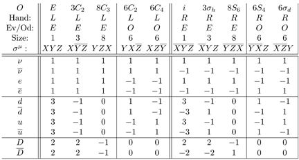(46)

In the above table, the five columns on the left are the left handed or proper rotations, and the five columns on the right are the right handed or improper rotations. Each of these five columns are split into three even and two odd columns.

We can write the operator for electric charge Q in terms of the classes of the Geo43 group. That is, Q is a diagonal operator in $43\left[{\sigma }^{\mu }\right]$ that commutes with all the irreps and so can be written as a sum

$Q={\Sigma }_j{q}_j{I}_j$ (47)

where $q_j$ is the electric charge of the jth particle, and $I_j$ is the identity for the corresponding block on the diagonal. The blocks on the diagonal correspond to the irreps of the original character table and so each $I_j$ can be written as a sum of products of the group classes. These can be read off of the character table as shown in the previous section. As always occurs with character tables, the number of irreps is the same as the number of classes (columns) so there is only one choice for the electric charge operator when writing it as an element of $43\left[{\sigma }^{\mu }\right]$.

Since particles and anti particles have opposite electric charge, examining the table shows that the Q operator can be composed only of right handed elements. The left (right) handed particles will be composed only of left (right) handed elements so their weak isospin and weak hypercharge will depend only on left (right) handed group elements. Weak hypercharge for right handed particles is the same as electric charge which we already know is made only of right handed elements. This reduces the algebra needed to define the charges to be a 5 × 5 transformation instead of 10 × 10. Writing the left and right handed elements of the particles in the same columns we have:

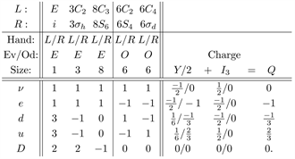(48)

When the classes in the above table are expanded to the elements the five columns will increase to $1+3+8+6+6=24$ and the operators are obtained by dividing by 24. We will do the algebra without this division and insert it at the end. Also, in the above table there is a subtlety on the scaling. The projection operators for the quark identities 1₃ is three times the amount shown. This would require us to multiply those rows by three, but these projection operators apply to three colors of quarks while the experimentally measured charges are for a single quark so we also need to divide by three.

Right weak isospin is always zero, and charge is the same as right weak hypercharge leaving us three equations to solve: left and right weak hypercharge, and left weak isospin. Left weak hypercharge depends only on the even left components giving three equations in three unknowns:

$\begin{array}{l}1Y/2^E+1Y/2^{3C2}+1Y/2^{8C3}=-1/2\mathrm{,}\\ 3Y/2^E-1Y/2^{3C2}+0Y/2^{8C3}=1/6\mathrm{,}\\ 2Y/2^E+2Y/2^{3C2}-1Y/2^{8C3}=0.\end{array}$ (49)

Left weak isospin depends only on the odd left components so there are two equations in two unknowns:

$\begin{array}{l}1I_3^{6C2}+1I_3^{6C4}=1/2\mathrm{,}\\ 1I_3^{6C2}-1I_3^{6C4}=-1/2\mathrm{.}\end{array}$ (50)

Electric charge and right weak hypercharge use all five right components giving five equations:

$\begin{array}{l}1Y/2^i+1Y/2^{3\sigma h}+1Y/2^{8S6}+1Y/2^{6S4}+1Y/2^{6{\sigma }_d}=0,\\ 1Y/2^i+1Y/2^{3\sigma h}+1Y/2^{8S6}-1Y/2^{6S4}-1Y/2^{6{\sigma }_d}=-1,\\ 3Y/2^i-1Y/2^{3\sigma h}+0Y/2^{8S6}+1Y/2^{6S4}-1Y/2^{6{\sigma }_d}=-1/3,\\ 3Y/2^i-1Y/2^{3\sigma h}+0Y/2^{8S6}-1Y/2^{6S4}+1Y/2^{6{\sigma }_d}=2/3,\\ 2Y/2^i+2Y/2^{3\sigma h}-1Y/2^{8S6}+0Y/2^{6S4}+0Y/2^{6{\sigma }_d}=0.\end{array}$ (51)

Solving these linear equations for the operator coefficients defines the operators as

$\begin{array}{cccccccc}{I}_3& =& 0& 0& 0& 0& +12\left(6C_4\right),& \text{Left}\\ Y/2& =& 0& -4\left(3C_2\right)& -8\left(8C_2\right)& 0& 0& \text{Left}\\ & & 0& -4\left(3{\sigma }_h\right)& -8\left(8S_6\right)& 0& +12\left(6{\sigma }_d\right),& \text{Right}\\ Q& =& 0& -4\left(3{\sigma }_h\right)& -8\left(8S_6\right)& 0& +12\left(6{\sigma }_d\right),& \text{Right}\end{array}$ (52)

where the terms have been arranged according to their symmetry and their left and right elements are labeled to the right side. The coefficients are for the class; we could have divided by the size of each class and obtained charges per group element of −4/3 for $\left(3C_2\right)$ and $\left(3{\sigma }_h\right)$, −1 for $\left(8C_2\right)$ and $\left(8S_6\right)$, and +2 for $\left(6C_4\right)$ and $\left(6{\sigma }_d\right)$.

In mapping the irreps to the particles we had freedom in that we could independently swap the leptons and swap the quarks. This would change some of the signs in the −4 and −8 columns as well as swapping $\left(6C_4\right)$ for $\left(6C_2\right)$ and $\left(6S_4\right)$ for $\left(6{\sigma }_d\right)$.

Since charge does not commute with handedness, the equation $Y/2+I_3=Q$ requires an assumption not obvious in the above: it follows when one uses Q as the charge of a Dirac bispinor so that the particle portion has charge Q while the antiparticle portion has charge −Q.

For low temperatures, a heat bath is typically conceived as an object that can exchange electric field gauge bosons (i.e. heat photons) with the system under study. However, when we model such a system with density matrices the gauge bosons do not appear explicitly; their effect is implicit. The gauge boson for the weak force is the $W^{\pm }$. As the temperature rises above the amount needed to create $W^{\pm }$ gauge bosons, it becomes possible for the heat bath to convert between electrons and neutrinos, and to convert between up quarks and down quarks. In the temperature flow shown in Figure 1, we can see that the cooling states clump together into curving arcs. These occur because certain degrees of freedom cool faster than others. We can imagine that these correspond to a cascade of symmetry breaking from the high temperature limit where all states are approximately identical. Then the weak symmetry breaking is the coolest of these.

5. Generations

While the group algebra Geo43 discussed in the previous section includes a single generation of the Standard Model fermions, to include the generation structure requires that we use a finite group that has three times as many degrees of freedom. The finite Abelian group of size 3, $C_3$, is perfect for this. To define this group we will use the complex cubed root of unity

$\omega =exp\left(2i\pi /3\right)\mathrm{.}$ (53)

So the group elements are $\left\{\mathrm{1,}\omega \mathrm{,}{\omega }^{\mathrm{<mo>\; *\; </mo>}}\right\}$ and the group product is the usual for complex numbers. The character table for $Z_3$ is:

$\begin{array}{cccc}{C}_3& 1& \omega & {\omega }^{\mathrm{<mo>\; *\; </mo>}}\\ A& 1& 1& 1\\ E& 1& \omega & {\omega }^{\mathrm{<mo>\; *\; </mo>}}\\ E^{\mathrm{<mo>\; *\; </mo>}}& 1& {\omega }^{\mathrm{<mo>\; *\; </mo>}}& \omega \end{array}$ (54)

Since this is an Abelian group, the three classes correspond to the three elements of the group and the character table defines a discrete Fourier transform.

When we multiply a finite group by an Abelian finite group the character table of the new group is the product of the two character tables. Thus when we triple Geo43 with $C_3$ to form the modified point group we call 3Geo43 it will have 30 classes instead of the 10 that Geo43 had, and it will have 30 irreps as well. Each of the old Geo43 irreps will appear in the new character table three times, once with $\left(\mathrm{1,1,1}\right)$ as the characters of $\left(\mathrm{1,}\omega \mathrm{,}{\omega }^{\mathrm{<mo>\; *\; </mo>}}\right)$, again with characters $\left(\mathrm{1,}\omega \mathrm{,}{\omega }^{\mathrm{<mo>\; *\; </mo>}}\right)$ and finally with characters $\left(\mathrm{1,}{\omega }^{\mathrm{<mo>\; *\; </mo>}}\mathrm{,}\omega \right)$. Thus $\nu$ will now appear three times, once with thirty 1s, once with ten 1s, ten $\omega$ s and ten ${\omega }^{\mathrm{<mo>\; *\; </mo>}}$ s, and finally the same but with $\omega$ and ${\omega }^{\mathrm{<mo>\; *\; </mo>}}$ reversed.

The character table of 3Geo43 will be of size 30 × 30 and is larger than we can reasonably print in a journal. There will now be 144 Weyl equations to decouple with a total of $2\times 4\times {144}^2=165888$ terms but the equations will uncouple according to the character table as before and the result will be three copies or generations of the Standard Model fermions.

Given that the character table of $C_3$ defines the generation structure, it’s natural to look for a dependency on those characters in experimental data that depends on generation. The most obvious of these are how the masses of the Standard Model fermions depend on the generation and indeed, this is precisely what is seen in the Koide formulas for the lepton and quark masses [12] [13] [14]. Other generation structures, such as the CKM and PMNS matrices that define how the weak force converts between generations will be more complicated in that they must depend on both the $C_3$ and Geo43 character tables and formulas for those have not yet been found.

6. Dark Matter Nomenclature

The extra “dark matter” irreps, D and $\bar{D}$ in the $43\left[{\sigma }^{\mu }\right]$ character table of Equation (46) have zero electric charge, weak hypercharge and weak isospin and so do not participate in the electric or weak forces. In the Standard Model, the color force is determined by quark SU(3) internal symmetries. In this model, the quark SU(3) operators are internal to the quark irreps in that they act on the traceless degrees of freedom in the 3 × 3 quark blocks. The remaining degree of freedom is the 3 × 3 unit matrix which is the projection operator proportional to the usual irrep. These quark SU(3) color degrees of freedom are restricted to the corresponding quark 3 × 3 blocks so they annihilate between different quarks.

Examining the character table we see that the quarks differ in the signs of their odd elements, $\left(6C_2\right)$, $\left(6C_4\right)$, $\left(6S_4\right)$ and $\left(6{\sigma }_d\right)$ therefore the gluons must be associated with changes in these elements. But the dark matter irreps are zero in those columns so they cannot participate in the strong force. Thus the dark matter irreps are indeed dark.

As with the leptons and quarks, dark matter comes in particle D and antiparticle $\bar{D}$ form and appears in three generations. They differ in sign between the left and right handed parts of the particles as do the leptons and quarks so we expect that dark matter will also have mass.

The dark matter irreps have an internal SU(2) symmetry that is otherwise similar to the quark’s internal SU(3) symmetry. By analogy with the quarks, we will label the dark matter SU(2) internal symmetry as colors. As the dark matter particles that correspond to quarks, we will call them “dark quarks” or “duarks”. Since these have only an SU(2) symmetry, there are only two dark colors needed as a basis for dark color. Where the colors for quarks are expressive of their participation in electromagnetic photon interactions, the duarks are dark so in contrast to the quark colors of red, green and blue, we will use dark colors of “doom” and “gloom”. These are also appropriate for this paper which is being written under the looming threat of the Covid19 pandemic.

We assume that there is a force boson similar to the gluon between them, call it the “duon”, that will follow an SU(2) triplet symmetry. Where the eight gluons are often described using a basis of the eight Gell-Mann matrices, the three duons can use the three Pauli matrices to define the dark matter triplet:

$\begin{array}{l}\left(d\bar{g}+g\bar{d}\right)/\sqrt{2}\mathrm{,}\\ -i\left(d\bar{g}-g\bar{d}\right)/\sqrt{2}\mathrm{,}\\ \left(d\bar{d}-g\bar{g}\right)/\sqrt{2}\end{array}$ (55)

where d and g stand for the doom and gloom dark colors. The presence of a gluon-like force implies that dark matter has a significant scattering cross section with itself. This possibility is in the literature described as “self interacting cold dark matter” or SICDM [14].

A quark and an antiquark can combine to form a meson; we expect that a duark and an antiduark similarly combine to form a “deson”. While the mesons decay by electroweak processes, the desons do not participate so we may suppose that they are stable. Similarly, three quarks can combine to form a baryon so two duarks of different dark colors, combine to form a “daryon”.

Acknowledgements

We hope that the reader has enjoyed reading this paper even more than the author enjoyed writing it. Of course the author has received assistance from many physicists. Of particular note are his advisors in the physics program at Washington State University, Michael Forbes, Sukanta Bose and Fred Gittes. Their interest and encouragement were critical to maintaining the long effort required here. And that long effort was too long by two or three years as WSU has a limitation on how long one can take to write a thesis. The author thanks his advisors for continuing to assist after that time ran out. The author hopes that the university will find a way of making an exception and that this paper will be considered as a partial fulfilment of the PhD degree in physics at WSU.

Conflicts of Interest

The author declares no conflicts of interest regarding the publication of this paper.

References

[1]	Peskin, M.E. and Schroeder, D.V. (1995) Introduction to Quantum Field Theory. Addison-Wesley Pub. Co.
[2]	Hestenes, D. and Holt, J.W. (2007) Journal of Mathematical Physics, 48, Article ID: 023514. https://doi.org/10.1063/1.2426416
[3]	Terras, A. (2012) Harmonic Analysis on Symmetric Spaces and Applications I. Springer Science & Business Media, Berlin.
[4]	Mackey, G.W. (1980) Bulletin of the American Mathematical Society, 3, 543-698. https://doi.org/10.1090/S0273-0979-1980-14783-7
[5]	Steinberg, B. (2012) Representation Theory of Finite Groups: An Introductory Approach. Springer, Berlin. https://doi.org/10.1007/978-1-4614-0776-8
[6]	Patrignani, C., et al. (2016) Chinese Physics C, 40, Article ID: 100001. https://doi.org/10.1088/1674-1137/40/10/100001
[7]	Roe, B.P. (1996) Particle Physics at the New Millennium. Springer-Verlag, New York. https://doi.org/10.1007/978-1-4612-2362-7
[8]	Dreiner, H.K., Haber, H.E. and Martin, S.P. (2010) Physics Reports, 494, 1-196. https://doi.org/10.1016/j.physrep.2010.05.002
[9]	Hamermesh, M. (1962) Group Theory and Its Application to Physical Problems. Dover, Mineola. https://doi.org/10.1119/1.1941790
[10]	Brannen, C.A. (2010) Foundations of Physics, 40, 1681-1699. https://doi.org/10.1007/s10701-010-9465-8
[11]	Sheppeard, M. (2009) Rejecta Mathematica, 1, 104-110.
[12]	Zenczykowski, P. (2012) Physical Review D, 86, Article ID: 117303. https://doi.org/10.1103/PhysRevD.86.117303
[13]	Brannen, C.A. (2006) Koide’s Mass Formula for Neutrinos. 8th Annual APS Northwest Section Meeting, Tacoma, 19-20 May 2006. http://meetings.aps.org/Meeting/NWS06/Event/50546
[14]	Spergel, D.N. and Steinhardt, P.J. (2000) Physical Review Letters, 84, 3760-3763. https://doi.org/10.1103/PhysRevLett.84.3760