The Contrastive Empirical Study of Social Financing Scale Increment and Stock ()
1. Introduction
The scale of social financing is a total indicator that reflects the relationship between finance and the economy and the financial support of the real economy. Based on the consideration of unified social financing scale in 2014, the People’s Bank of China released the first historical data on the scale of social financing stocks from 2002 to 2014, which indicates that the scale of social financing has become an important factor determining the direction and strength of monetary policy. The scale of social financing can be divided into two types: stock and increment. In the past, scholars have conducted more research on the increase of social financing scale. Among them, [1] [2] [3] studied the controllability of the increase in social financing scale. [4] [5] [6] [7] research on the increase of social financing scale as the intermediate target of monetary policy. However, there are few studies on the stock of social financing scale. In fact, compared with the increase, the stock of social financing scale is more closely related to the main economic indicators (see [8] [9]). So, as the intermediate target of monetary policy, does the stock of social financing scale play a greater role than increment? To this end, this article takes the scale of social financing as the research object, establishes a VAR model, studies the relationship between the increase, stock, and economic development under different economic conditions, and compares the impact of the increase and stock as intermediate targets of monetary policy on economic development degree.
2. Empirical Analysis
2.1. Data Selection, Source and Processing
This article selects the GDP and the consumer price index CPI that can best represent the economic situation as the final target variables of monetary policy. Since the People’s Bank of China only compiled data on China’s social financing scale since 2002, this article selects quarterly data from 2002 to the present, that is, the increase in social financing scale and social financing from the first quarter of 2002 to the first quarter of 2017. Scale stock, CPI and real GDP data (take the first quarter of 2002 as the base period), and record them as SZ, SC, CPI, GDP in turn. The data comes from the wind database and the National Bureau of Statistics. In order to avoid the possible heteroscedasticity of the data from affecting the test results, log the original sequence to eliminate possible heteroscedasticity. The log-logged sequences are recorded as LnSZ, LnSC, LnCPI, LnGDP.
2.2. VAR Model Establishment Process
2.2.1. Stationarity Test
In order to avoid the time series data being unstable and pseudo-regression, the stationarity test needs to be performed on the modeling series. In this paper, the ADF unit root test is used to test the stationarity of the series LnSZ, LnSC, LnGDP and LnCPI, and the lag order is selected by the SC criterion. The test results are shown in Table 1.
As can be seen from Table 1, none of the LnGDP, LnCPI, LnSZ, and LnSC sequences have passed the stationary test. First-order difference processing is performed on the above sequences, and the processed sequences are recorded as DLnSZ, DLnSC, DLnCPI, DLnGDP, and ADF unit root test is performed on these new sequences. The results are shown in Table 2.
![]()
Table 1. ADF test results of LnSZ, LnSC, LnGDP and LnCPI sequences.
![]()
Table 2. ADF test results of DLnSZ, DLnSC, and DLnGDP sequences.
From Table 2 above, it can be seen that after the first-order difference, each sequence has been stabilized, that is, the LnGDP, LnCPI, LnSZ, and LnSC sequences are all first-order simple integer sequences.
2.2.2. Determination of Model Order and Stability Test
For the VAR model, in practical applications, it is usually desired that the lag period is large enough to fully reflect the constructed dynamic characteristics. However, the longer the lag time, the more parameters to be estimated in the model and the less degrees of freedom. Therefore, a balance should be sought between lag time and degrees of freedom. EViews software provides the results of the most commonly used LR test statistics, final prediction error (FPE), AIC information criterion, SC information criterion, and HQ information criterion, and the optimal lag order selected according to the corresponding criterion is marked with “*” number.
Table 3 shows the LR, FPE, AIC, SC, and HQ values of the VAR model of order 0 to 7. The lag order selected according to the corresponding criteria is marked with “*”. It can be seen that the order chosen by the three criteria is 4th order, so the lag order of the model can be set to 4th order. Use EViews7.2 to build a VAR (4) model. The model estimation results are as follows:
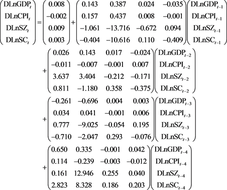 (1)
(1)
![]()
Table 3. Judgment results of lag order.
After estimating the model, the stability of the model needs to be tested. The AR root map and table of the model check are shown in Figure 1 and Table 4 below. It can be seen that the inverses of all equation roots are located in the unit circle, that is, the overall model has stability.
2.2.3. Co-Integration Test
Because the LnGDP, LnCPI, LnSZ, and LnSC sequences are not stable, that is, the horizontal sequence is not stable, it is not possible to directly establish a VAR model. However, the above ADF unit root test is known that these sequences are first-order single integer sequences. There is a stable long-term equilibrium relationship. If there is a cointegration relationship between the variables, the differential VAR model established above will be reasonable. Due to the optimal lag order of our VAR model, the lag order of the cointegration test here should be 3. Johansen cointegration tests were performed on the sequences LnGDP, LnCPI, LnSZ, and LnSC, the results are shown in Table 5 and Table 6 below.
From Table 3 and Table 4, it can be seen that the results of the rank test and the maximum characteristic root test of the Johansen cointegration test indicate that at a significance level of 5%, the LnGDP, LnCPI, LnSZ, and LnSC sequences have a cointegration relationship, that is, there is a long-term equilibrium relationship. The VAR model established for DLnGDP, DLnCPI, DLnSZ, DLnSC is suitable.
2.2.4. Impulse Response Function and Variance Decomposition
Without considering the large-scale economic changes (that is, in terms of the current state of our economy), the impulse response of GDP to the positive impact of the increment of social financing scale and the unit standard deviation of the stock is shown in Figure 2 and Figure 3 below. It can be seen that there is a one-phase (that is, one quarter) lag in the impact of GDP on the increase in social financing scale and stock. When a positive impact is given to the stock of social financing scale, the impact of GDP is the largest in the fifth period, and its value is greater than the increase in the size of the social financing scale. The positive impact of a unit standard deviation on GDP has the largest impact on the GDP. There is still an impact, and the impact of the increase on GDP basically continues to the 8th period, that is, the impact of the stock on GDP is longer than the increase, but the stock has a negative impact on GDP, and the increase has an impact on GDP in each period. It is a positive influence.
![]()
Table 4. AR root table of VAR model.
![]()
Table 5. Johansen co-integration rank test results.
![]()
Table 6. Results of Johansen co-integration maximum eigenvalue test.
![]()
Figure 2. Impulse response of DLnSZ to DLnGDP.
![]()
Figure 3. Impulse response of DLnSC to DLnGDP.
Variance decomposition is to further evaluate the importance of different structural shocks by analyzing the contribution of each structural shock to the change of endogenous variables. It can be seen from Table 7 that the contribution rate of the increase in social financing scale to GDP has slowly increased over time; the contribution rate of social financing scale stock to GDP has increased significantly during the fourth to fifth periods, The contribution rate of the stock to GDP is also slowly increasing, but the contribution rate of the stock to GDP is greater than the incremental contribution rate to GDP in the same lag period. It can be seen that the stock of social financing scale plays a greater role in the change of GDP.
![]()
Table 7. Contribution ratio of social financing scale increase and stock shock to GDP.
At present, China’s economy is operating steadily. After the above analysis, in general, the scale of the stock of social financing is more suitable as an intermediate target for monetary policy than incremental. But the intermediary goal of monetary policy should not only play a role when the economy is good and prices stable, but also it should play a role when the economy is depressed or inflation is severe. Therefore, in order to more objectively evaluate the advantages and disadvantages of the increase of social financing scale and stock as the intermediate target of monetary policy, the effects that the two can achieve under different economic conditions should be considered.
The following compares and analyzes the effects of the increase in the scale of social financing and the stock in the economic downturn and hyper-inflation.
1) Under economic downturn
During the economic downturn, the impact of the increase in the scale of social financing on the GDP (equivalent to DLnGDP applying a unit of negative impact and simultaneously DLnSZ applying a unit of positive impact) is shown in Figure 4 below. Impact, and apply a unit of positive impact at the same time) as shown in Figure 5, because Figure 4 and Figure 5 have similar trends, it is not easy to compare, so it is converted into a digital table for comparative analysis (see Table 8). It can be seen from Table 8 that due to a unit of negative pulse received by GDP itself, it has shown the negative effects of increment and stock on it in the first three periods, but the absolute value of negative effects is decreasing, indicating that Both stocks and increments have played a role. Until the 4th period, the positive impact of stock and increment on GDP exceeded its negative impact, that is, the impulse response to GDP showed a positive value, and the impact of stock on GDP was 0.137, which was higher than the incremental impact. The GDP shock was 2.3 percentage points, which indicates that the stock has a greater positive impact on GDP compared to the increase.
![]()
Table 8. Impact of Increment and Stock on GDP during Economic Downturn.
2) In the case of hyperinflation
In the case of hyper-inflation, the increase in the scale of social financing (equivalent to a positive impact on both LnCPI and DLnSZ), the impact on CPI and GDP is shown in Figure 6 and Figure 7. When the stock is increased during hyperinflation (equivalent to applying a positive shock to both DLnCPI and DLnSC), the impact on CPI and GDP is shown in Figure 8 and Figure 9 below. It can be seen that starting from the second period, the increase and stock began to have an effect on CPI and GDP, that is, it showed the lag of the first period, and the impact gradually weakened and reached zero from the fifth period. Similarly, for comparison, the impulse response graph is converted into a table for analysis. As can be seen from the impulse responses in Figure 6, Figure 8 and Table 9, the impact of CPI is getting smaller and smaller, and in the fifth period, both the increase and the stock have negative effects on the CPI, showing that both the increase and the stock have stable prices Role. In the fifth period, the stock’s impact on CPI is −0.329, and its absolute value is higher than the negative impact of incremental growth on CPI (−0.316). The absolute value is 1.3 percentage points, that is, the effect of stock stability on prices is slightly higher than the increase; Looking at the impact of the impact, the positive impact of the incremental increase on GDP in the second period is 0.411, which is greater than the impact of the stock on the same period (0.352) by 5.9 percentage points. In addition, the positive impact of the incremental increase on GDP in the third period. The shock (0.413) is 1.6 percentage points greater than the shock to GDP of the stock (0.397). That is, under hyperinflation, the increase has a greater stimulating effect on GDP than the stock.
![]()
Table 9. Impact of Increment and Stock on GDP and CPI during Inflation.
![]()
Figure 6. Impulse response graph of increment to CPI during hyperinflation.
![]()
Figure 7. Impulse response of GDP to GDP during hyperinflation.
![]()
Figure 8. Impulse response of stocks to CPI during hyperinflation.
![]()
Figure 9. Impulse response of stocks to GDP during hyperinflation.
3. Conclusion
Based on the above three different situations of stable economic operation, economic downturn, and hyperinflation, the comparative analysis of the impact of the increase in social financing scale and stock on the economy can be concluded as follows: 1) According to the results of the Johansen cointegration test, there is a long-term stable equilibrium relationship between GDP, consumer price index, social financing scale increase, and stock. 2) In the case of stable economic operation, according to the impulse response function, from the perspective of the impact degree, the effect of the social financing scale stock on the economy is better than that of the incremental economy. From the results of variance decomposition, the stock plays a greater role in the change of GDP. 3) In the economic downturn, both the stock and the increase have played a good role in the economy, and from the comparison of the impulse response chart, it is seen that the stock has a greater positive impact on GDP than the increase. 4) When hyperinflation occurs, both the increase and the stock have the effect of stabilizing prices, and the stability of the stock on prices is slightly higher than the increase, but the increase has a greater stimulating effect on GDP. 5) From the impulse response diagrams in the three cases, it can be seen that there is a certain time lag effect on the impact of the increase and stock of social financing scale on GDP and prices in any case, from the expansion of social financing scale to its impact. There is a period of conduction.
Funds
This work is supported by the National Natural Science Foundation of China (No. 11561056) and Natural Science Foundation of Qinghai (No. 2016-ZJ-914).