Resolution of Grandi’s Paradox as Extended to Complex Valued Functions (Editorial)
1. Introduction
Luigi Guido Grandi (1671-1742) is known due to his book entitled Quadratura in short. The book does not contain much original work except for two particular items; namely, the construction of a curve that has become known as the Witch of Agnesi and the identification of a paradox originating from the series expansion of
. Through Grandi’s personal correspondence with the well-known mathematicians, such as Leibniz (1646-1716), the paradox has gained a renown and in time named after Grandi [1]. The paradox can be stated as follows. Consider the series expansion of
, which may be obtained by performing a simple division or expanding into a Maclaurin series. Both methods give the same result,
(1)
which obviously converges for
and diverges for
. The upper limit of convergence,
, is named here as the threshold point for later purposes. Grandi remarked that for
the left-hand side of (1) would be
while the right-hand side could be collected as
, so that one would end up with the paradox
.
Before proceeding to the resolution of the paradox the series expansion in (1) is rendered convergent for
by a simple manipulation as follows
(2)
Since
for
, (2) is convergent for
.
2. Resolution of Grandi’s Paradox
In tackling with Grandi’s paradox the crucial point is to perceive the duality embedded in it. Starting from this recognition the paradox can be resolved as presented in detail in Beji [2]. Here, we shall first recapitulate the main aspects of that work and then proceed to extend it to complex valued functions.
The duality concerns the numerical value of series expansion depending on the number of terms included for the threshold value
. If one retains terms up to an odd power in the series,
(3)
where n is an arbitrary integer, the resultant sum on the right is obviously 0 for
. On the other hand, if terms up to an even power are kept,
(4)
setting
results in 1 on the right. Thus, depending on the highest power kept being odd or even the result on the right is either 0 or 1. In a sense, the series cannot be called precisely convergent for
. The paradox indeed pivots around this altercation of numerical values. The resolution must introduce a reconciliation such that taking just one more term should not result in any appreciable difference for
.
Figure 1 presents a visual demonstration of the dual character of Grandi’s paradox for different truncation orders. Note that different truncations produce
![]()
Figure 1. Visual demonstration of the duality of Grandi’s paradox for
. Function
(black line) and its standard series expansions truncated at different orders.
respectively 0 and 1 for the threshold point
but not the correct value 1/2. For this reason, series representations diverge rapidly either to 0 or 1 from the actual function
in the vicinity of
. Equations (1) and (2) are used to plot the series expansions for
and
, respectively.
To reconcile the results of expressions with different truncation orders we must combine Equations (3) and (4). Multiplying each expression with an arbitrary constant and adding side by side by is the only operation that would not alter the left hand side. Thus, Equation (3) is multiplied with
, Equation (4) with
and added side by side. Setting
in this expression and imposing
for keeping the left-side unchanged give
. This corresponds to the case with odd highest power in the series. The same line of approach may be followed when the highest power is even. The resulting expressions read:
(5)
(6)
Accordingly, if the series is truncated by taking the one-half of the last term, the correct result 1/2 is obtained for the threshold point
, regardless of the truncation order. The resolution presented may at first sight appear as an ad hoc approach specifically devised to obtain the desired result; nevertheless, its soundness shall be more evident with further ramifications and different applications, as d’Alembert (1717-1783) said on the defence of calculus: “Allez en avant, et la foi vous viendra1”.
The consistent truncation introduces a corrective collocation which improves the numerically computed value of the function from the series expansion. For instance, setting
in the function
and the usual series expansion to the fourth-order gives respectively
and
. The corresponding relative error is
, which is 32.7%. On the other hand, using the
consistent truncation gives
, which is
−4.1% in error. The improvement is appreciable but it is possible to do much better as described next.
3. A Convergence Improvement Technique
A technique for improving the convergence properties of truncated series is now introduced. The approach is demonstrated for the series expansion of
but it can be generalized quite easily and applied to any series expansion as shown later. The technique proceeds by taking successive averages of the consis-
tent truncations of the first-order,
, of the second-order
and
of the higher-orders. Table 1 shows the method for the series expansion to the fourth-order.
Procedure is carried out by averaging the consistently truncated expansions at successive orders; that is,
is added to
and the result is averaged to get
. The ultimate result of this process is the fourth-order expansion
, which, like each individual expression
in the table, satisfies the threshold condition 1/2 when
. For the previously considered case of
, the value rendered by this fourth-order expression is now 0.556 and identical with the exact value
to the third decimal point. The improvement is virtually enormous. The approach demonstrated in Table 1 for a definite number of terms can be generalized to an arbitrary number of terms.
![]()
Table 1. Successive averaging of the consistently truncated series expansions of
.
(7)
For
Equation (7) can be put into the following convergent form by the approach used in Equation (2):
(8)
in which the truncation order n may be selected as an odd or even integer. The most striking feature of the series expansions (7) and (8) is the change of coefficients depending on the truncation order. For a given truncation the coefficients are adjusted in a way to yield a highly accurate representation of the generating function. This special aspect is the principle novelty of the consistent truncation and successive averaging approach.
Figure 2, which may be viewed as the counterpart of Figure 1, shows the plots
![]()
Figure 2. Function
and its consistently truncated and successively averaged series expansions.
of the series expansions given by Equations (7) for
and (8) for
. Series of four different truncation orders are compared with the generating function
within the range
. Except for the second-order truncation, which stands out slightly, all the others are in virtually perfect agreement with the function
itself for the entire range shown and obviously it is so for
. Figure 2 actually represents a visible demonstration of the resolution of Grandi’s paradox.
Integration of (7) and (8) would result in fast converging series representations of the natural logarithm function.
(9)
(10)
Note that when
,
on the left grows boundlessly while the terms involving the powers of 1/x on the right go to zero. But
, arising from the integration of the first term 1/x on the right-side of Equation (8), takes care of this problem. An important point in using (9) and (10) together for computations is to dismiss the highest-order term
in (9) completely to be consistent with the highest-order term
in (10). This crucial aspect is numerically demonstrated for
in Beji [2].
4. Mathematical Justification of Consistent Truncation and Convergence Improvement Techniques
In order to resolve Grandi’s paradox in a suitable way, we have first introduced a consistent truncation approach and then a convergence improvement technique of successive averaging. While the satisfactory outcome of these procedures itself is a justification enough, relating both applications to a solid mathematical background is desirable.
Grandi’s function
is now written in the extended form
with
. Carrying out a simple division gives
(11)
which obviously produces a paradoxical result for
, exactly in line with Grandi’s case. Expressing all the exponential functions in Equation (11) as Maclaurin series truncated at the fourth-order gives
(12)
After re-arranging the like-terms one obtains
(13)
which results in
when
. If Equation (11) is truncated after
, Equation (13) turns out to be
, which gives 1/2 = 0
when
. Again, just like Grandi’s paradox, depending on the number of terms kept, a duality of results is observed. However, despite all these similarities, the function
has a different property compared to
. A direct expansion of
into a Maclaurin series produces
(14)
which correctly satisfies
when
. We are then facing an interesting case of two different approaches aimed at the same end but producing conflicting results. Obviously, Equation (14) is the correct result and if it can be obtained by employing the method applied to resolving Grandi’s paradox we can claim a solid background for our approach. Thus, we begin with Equation (11) but apply the consistent truncation procedure followed by successive averaging as exactly done for the sample calculation given in §3, Table 1. Without repeating all those steps we simply set
in place of x in Table 1 and obtain
(15)
which is strictly truncated at the fourth-order as all the coefficients are determined according to this truncation order. Substituting the fourth-order Maclaurin series for the exponential functions, as we did to Equation (11), gives
(16)
Collecting the terms of the same order together gives
(17)
which, except for the fourth-order term, is essentially the same as Equation (14). The disagreement in the fourth-order terms originates from the difference between the classical infinite series formulation and the truncated approach embedded in the present method. If a fifth-order expansion were carried out the fourth-order terms would be identical while the fifth-order terms are different. Only for infinitely many terms would the present approach be identical with the classical one as the coefficient of the highest-order term tends to zero. This demonstration has thus revealed a subtle connection between the classical Maclaurin series expansion of a function and the consistent truncation and successive averaging technique introduced here to resolve Grandi’s paradox. Such a far-fetched connection is unexpected but quite satisfying as it bolsters confidence in the method by providing firm theoretical support.
5. Grandi’s Paradox for Complex Valued Functions
We now proceed to define complex valued functions which yield paradoxical results for definite x values when expanded into series just like
. The function
would serve as a good starting point for extending the procedure to the complex domain. First, we note that
(18)
where
is the imaginary unit. Our primary aim here is to carry out a consistent truncation and convergence improvement of the series expansions of
and
. Before proceeding towards this goal it is appropriate to apply these methods to
so that the results can be used to establish the expansions of
and
.
The standard series expansion of
is
(19)
Obviously, the right-hand side of Equation (19) produces paradoxical results for
. Without repeating the entire procedure the consistently truncated and convergence improved form of Equation (19) is obtained by simply setting
in place of x in Equation (7). Thus, the general formulations are
(20)
(21)
where n is an arbitrary truncation order.
At this stage, it is tempting to compute estimated π values by use of the standard and improved series expansions of
. Let us keep up to and including the tenth power as in Equation (19) for the standard series. The corresponding improved expansion is obtained from Equation (20) by setting
:
(22)
Integrating (22) from 0 to 1 yields
(23)
Since
we get the following estimates from the standard and improved series
(24)
(25)
which have respectively −5.3% and 0.1% relative errors. The present improved series performs remarkably well compared to the standard approach. The same result could also be obtained from the integration of Equation (21), which is valid for
. However, care should be observed in setting the integration limits from 1 to
in the validity domain of the expansion. The left side then would be
. On the other hand, the right side at the upper limit would go to zero while at the lower limit would be multiplied by a minus sign, resulting in a correct positive estimate for π/4. Finally, of historic significance, it must be indicated that Equation (24) is originally due to Leibniz (1646-1716) [3], p. 10.
We now proceed to the treatment of
, one of the fractions making up
as given in (18). First note that
, hence the problem can be carried out separately for the real and imaginary parts. Equations (20) and (21) already give the improved series of
, which corresponds to the imaginary part. Multiplying (20) and (21) by
would simply produce the improved series of
, which corresponds to the real part. We must however observe that the real and imaginary parts have respectively odd and even powers of x and therefore truncation orders must be different for each part. Moreover, for exact result at the threshold point
the truncation power of the real part must be less than the imaginary part for
and vice versa for
. This arrangement of truncation orders has the additional advantage of giving exact functional value for
, just like a second threshold point. Bearing these precautions in mind we write down the consistently truncated and successively averaged series representation of
as follows.
(26)
(27)
The corresponding series for
can be directly written down by reversing the sign of i in the above equations. Numerical examples of Equations (26) and (27) truncated at a definite n value are now presented for demonstration purposes. Setting
results in
(28)
(29)
First, we set
the threshold point in both (28) and (29):
(30)
(31)
which both are exact. Next we try
:
(32)
(33)
which both are exact again. Thus, both expansions for
and
produce identical and correct results for the imaginary threshold point
and additionally for what might be termed the real threshold point
. On the other hand, the standard expansion obtained by division or Maclaurin series
(34)
would produce various paradoxical results for
and
, depending on the truncation order.
Figure 3 depicts the function
(red line), its standard series expansion, Equation (34) for
and its manipulated form for
, (green line), and consistently truncated and successively averaged series expansion (blue line) given by Equations (28) for
and (29) for
. In drawing the graphs x is given only real numbers within the range
in the vertical axis and the corresponding real and imaginary functional values are marked in the horizontal axes. The most remarkable aspect of the figure is that the graph of the function itself
drawn in red colour is virtually inseparable from the graph of (28) and (29) drawn in blue colour. The standard expansion drawn in green on the other hand exhibits its discontinuous character at
as in Figure 1.
![]()
Figure 3. Function
(red), its standard series expansion (green), and consistently truncated and successively averaged series expansion (blue). Series expansions are computed for
.
We end this section by establishing the Fagnano (1682-1766) formula [1]
from Equation (28) and its variant. Integrating (28) from 0 to 1 yields
(35)
can be obtained by changing the sign of i in (35):
(36)
Subtracting Equation (35) from (36) side by side gives
(37)
Recalling that
and evaluating the right-hand side numerically, Equation (37) becomes
(38)
Multiplying both sides by 2i and rearranging give
(39)
in which the right-hand side is in 0.04% error compared to π. The absolute error is approximately π/2500 and the convergence rate of the series expansion with only
terms is excellent. Notice that the calculation of π in Equation (25) is actually
case of (37).
6. A General Complex Valued Function and Its Special Cases
A complex valued function of a quite general form is now introduced:
(40)
(41)
where
and
are real quantities defining a given complex constant,
is a positive integer, and x is the independent variable which may be real, imaginary or complex. Obviously, Equations (40) and (41) result in a Grandi-type paradox, the series expansions producing values in conflict with the function for the threshold point
. We resolve the paradox by applying the consistent truncation approach and then carry out successive averaging technique for improving the convergence characteristics of the series. The resulting expressions, which correspond to (40) and (41), are
(42)
(43)
Equations (42) and (43), having the unusual features of power series interlaced with Fourier series, contain all the previously treated forms as special cases; however, care must be observed for terms alternately multiplied by zero values of cosine and sine functions. These regular zero multiplications, which occur for pure imaginary
values, must be excluded from the successive averaging process of a definite p value; instead, the next non-zero term must be taken in its place. These points are demonstrated clearly in the following examples.
6.1. Grandi’s Function
and
First, the improved series expansions of Grandi’s function
are obtained from Equations (42) and (43) as special cases. Setting
,
, and
in (42) and (43) yields respectively
(44)
45)
which are identical with Equations (7) and (8). The series corresponding to
can be readily obtained by setting
instead of
. Simply, replacing x by
in (44) and (45) results in (20) and (21).
6.2. Complex Valued Arbitrary Functions
and
We first recover the series expansions of
given by (26) and (27) from (42) and (43) as special cases. Substituting
,
, and
in (42) and (43) gives
(46)
(47)
For
Equations (46) and (47) become
(48)
(49)
It can easily be verified that both (48) and (49) render the threshold value −i/2 exactly for the threshold point
. Convergence improved series expansion of a function with a pure imaginary threshold point such as
is not unique and a different arrangement of Equations (46) and (47) is possible. First, the terms multiplied by zero can be skipped; specifically, those multiplied by
,
, etc. and
,
, etc. as appear in (48) and (49). Also, since the first term
in (48) is zero the first non-zero term of the
summation
is taken out as the leading term with av-
eraging coefficient of unity in accord with Table 1. With this particular term out, the first summation in (48) must now end at
instead of n to keep the truncation orders the same. Then applying a similar approach to (49) and properly changing the indices to skip the terms with zero coefficients results exactly in Equations (26) and (27). As shown before these equations have the advantage of yielding the correct functional value for
besides
. The case
can be handled similarly by setting
instead of
.
Finally, we consider a function in which the constant
is not real or pure imaginary but complex; that is,
and
hence
, and we set
so that the function is
. Using Equations (42) and (43) gives
(50)
(51)
Truncating the above expansions at
results in
(52)
(53)
The threshold value
, which is
for the present case, is now substituted into (52) and (53):
(54)
(55)
Right-hand sides of Equations (54) and (55) both yield the correct functional value
.
7. An Unorthodox Application of Successive Averaging Method
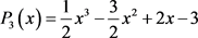
Successive averaging method, which has been used for improving the convergence characteristics of the series is now applied to a polynomial to generate a family of polynomials with equal and lower orders that approximate the generic one to varying degrees in the neighbourhood of .
.
The method can be best explained by an example. Let us consider a fourth-order polynomial with known roots  . The averaging process shown in Table 2 is exactly in line with Table 1; only now the terms making up the polynomial are used.
We have then generated the family of four polynomials ,
,  ,
,  , and
, and 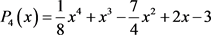 from the polynomial
 by successive averaging method. Figure 4 depicts all these polynomials, including the generating fourth-order polynomial. As observed, the newly generated polynomials are establishing a family of polynomials approximating to the generic polynomial in the neighbourhood of
 .
.
Use of the lower-order polynomials to estimate at least a root of the generic polynomial might be a conceivable idea. In the present case for instance  , corresponding to the last two terms of the generic polynomial, gives
 , which is 50% in error compared to the true root
 ; hence not good at all. Nevertheless, the averaging approach may be used to obtain better approximations in a definite neighbourhood to a series representation of a given function as demonstrated in [2]; its further applications may be discovered in the future.
![]()
Table 2. Successive averaging of a fourth-order polynomial for generating a family of polynomials.
![]()
Figure 4. Polynomial  (black) and the family of polynomials generated from.
8. Concluding Remarks
Resolution of the paradox originally posed for the series expansion of ![]() has been extended to Grandi-type complex valued functions of the form
has been extended to Grandi-type complex valued functions of the form ![]() . The method begins with a consistent truncation followed by successive averaging for improving the convergence characteristics of the power series considered. Theoretical support for this methodology is provided via a demonstration using different series expansions of the function
. The method begins with a consistent truncation followed by successive averaging for improving the convergence characteristics of the power series considered. Theoretical support for this methodology is provided via a demonstration using different series expansions of the function![]() . Fagnano’s formula is recovered in a non-trivial way by making use of the consistently-truncated and convergence-improved series expansions of
. Fagnano’s formula is recovered in a non-trivial way by making use of the consistently-truncated and convergence-improved series expansions of ![]() and
and![]() . In closing, an unorthodox use of the successive averaging method to polynomials is presented for suggesting diverse application areas.
. In closing, an unorthodox use of the successive averaging method to polynomials is presented for suggesting diverse application areas.
NOTES
1Go forward, and faith shall come.