Study of the Interception Scheme Based on A* Path Finding Algorithm in Computer Game ()
1. Introduction
AI, which can greatly promote the game play and the realism of computer games, is now one of most important topics of game design. This paper concerns about the interception problem in many aspects of the research of AI.
Before we discuss the interception issue, the pathfinding problem and the tracing problem should firstly be acquainted. pathfinding simply refers to the progress of searching an optimal path between two points. Many algorithms such as Dijkstra algorithm and Greedy algorithm are capable to finishing this task [1], and A* algorithm, proposed by P. E. Hart, N. J. Nilsson and B. Raphael, is the most widely used one. There will be a brief description about A* algorithm in the following context.
Based on A* algorithm, the study by [2] in 2017 has summed up the researches on dynamic pathfinding and the study [3] showed that the combination of Dynamic Pathfinding Algorithm, which proposed by [4], and A* Algorithm can provide a better effect than using A* Algorithm only.
Tracing problem refers to that when the demand of tracking a game unit B is put forward by another unit A, AI will seek an appropriate route for A. Many games use Sight-tracking algorithm to realize the tracing function. That is finding path from A to B and frequently changing the destination as well as path with the updating of target’s position and renewing of the game scene. The research about this algorithm been done by [5] in 2012. However, this method will make the game characters look stiff, especially when they need to show some kind of thinking ability. In that case, taking the way of chasing in real life as reference, on the basis of tracking algorithm, interception algorithm is developed to endow game characters with “intelligence”.
The existing solutions of interception problem are mostly the simple combination of dynamic pathfinding and A* Algorithm, which have a high requirement on the arrangement of scene, for instance, the algorithm applied to digital football game can only be used in an open field [6]. Thus we need a more general method to cope with dynamic obstacles and intricate terrains, also a more specific scheme for interception issue, and that is what this paper is going to be proposed.
The project is composed of three procedures, including choosing the way of interception, setting interception point and moving according to the found optimal path. In the process of this project, the authors propose the Known-Route-target Interception algorithm which is effective in intricate terrains. Meanwhile, in order to cope with dynamic obstacles, two algorithms improved from A*, which are named as Waiting Estimate algorithm and Known-Route-Obstacle A* algorithm here, are applied. Waiting Estimate algorithm cooperating with A* algorithm will enable AI of game to evaluate if it’s worthy to awaiting the dynamic obstacles, so that AI can decide whether to find a new path or just wait and detour. Known-Route-Obstacle A* algorithm makes the AI can take the obstacle with definite route into account so as to generate a barrier avoiding optimal path. What’s more, since the project is based on A* algorithm, with intent to save time spent on A* algorithm’s frequently invoking, a threshold value is introduced to the A* algorithm so as to promote it.
2. Conceiving and Problems
A basic prerequisite for interception is the dynamic state of the target. If target and interceptor are both dynamic, the key to interception should be predicting their moving progress separately. The interception process can be simply described as:
1) Deciding the means by which the interception is realized.
2) Using the corresponding algorithm of the chosen mean to find the interception point.
3) Targeting at the interception point, seeking optimal path and then moving along the path.
There may be some special cases. For example, sometimes obstacles can move. In this case, if the path of the dynamic obstacle is not considered, the path calculated in one time is likely to ignore some potential optimal path or lead to a collision.
According to the above analysis, the key to determining an interception scheme is to complete three tasks:
1) Find the interception point.
2) Determine the pathfinding method.
3) Decide the way to cope with dynamic obstacles.
3. Way of Interception and Target Setting
3.1. Interception in Game and Reality
In respect of interception, the examples in real world can be taken as reference. We will try to use police cars to intercept criminal in real life only when the criminal’s escape way is foreseeable, for example, the situation happening on expressway. In that case, each junction can be seen as a node. When executing interception, we just need to anticipate the target’s next arrived nod. However, in a chase that takes place in a neighborhood or on some busy street, the possibilities for movement are endless. So the path of the target is impossible to estimate, and chasing the target will be the main way. The last kind of situations based on an open area (e. s. in football games, interception in the air or on the sea) is special, in which the obstacles are no longer need to be given much thought to.
In order to analyze the first situation, we can scale down the space and time. The fork can be seen as a node and the road the link between two points. At the same time, the real time measure is scaled according to the time slice of the computer system. In this way, the interception on expressway can be regarded as the short-term and short-distance predict of interceptor toward the position of target in a graph. The space between the interceptor and the target is within a few points, and the distance will not greatly increase in a short time interval.
The second situation is actually a synthesis of interception issue and chase issue. Before the distance reaching to the range in which the interaction can take place, the interceptor will keep trying to approach the target. In certain circumstances, the interceptor can present predictability by predicting the next action of target, and thus turning chasing into interception.
In the third situation, the destination of target is known and the route is also predictable. The path of target will not radically changed because of barriers. In that case, the general interception method combined with obstacle eluding method will be suitable.
Certainly, for issue of interception, developers will hope to predicate the action of target. But with the increasing of distance, the possibility of target’s moving will also exploding exponentially. With the help of machine learning, AI may be able to calculate the respective probability of the different movements. But machine learning is beyond the scope of our discussion and will not be expanded.
3.2. Three Common Interception Method
In order to adopt different interception method, we need to analyze the existing interception algorithms first.
3.2.1. Destination Predict
The process of method is as follows:
The method simply set the destination of target as interceptor’s destination. This is corresponding to the first situation mentioned above.
The advantages of method:
The destination can be easily obtained without any complex calculation, thus can be frequently invoked.
The problems of method:
1) When the destination is very closed to interceptor but far away from target, the interceptor may wait for target at the destination.
2) Due to the speed change of the target is not taken into consideration, many useless roads may be taken when the target speed is changeable, which is not flexible enough. But because of the simplicity of the way it gets to the destination, it can update the intercept location every moment. And because it has better predictability than position prediction, its performance in short-range interception is better than the second method.
3) The accessibility of the target’s destination is a precondition, so its scope of application is limited.
3.2.2. Position Predict
The process of method is as follows:
This method is predicting the position of target in the next slice of time according to its speed and location, and then takes the predicted position as interceptor’s destination. It’s corresponding to the second situation mentioned above.
The advantages of method:
1) The necessary calculation is simple which can be quickly finished.
2) It guarantees that the interceptor can quickly approach the target in every time slice, so as to cope with the condition in which target’s speed is variable.
But due to the accessibility of destination, the interval of renewing can be shorten to every single time slice.
The problems of method:
1) The interception algorithm requires the interception location to be updated in every time slice, otherwise the interception cannot be completed, so it needs to be called frequently.
2) When tracking a distant target, the effect is not obvious which is similar to the line-of-sight tracking algorithm.
3.2.3. Interception Algorithm
The general process of the interception is as follows:
This algorithm firstly calculates the speed of the interceptor relative to the target with the speed of the interceptor and the target, then calculates the displacement between the two. Divide the displacement by the interceptor’s maximum rate to find out how long it will take to intercept, multiply the target’s current rate by time and then plus target’s position to find out where the intercept is about to take place. Finally, the pathfinding algorithm is used to make the interceptor move towards the interception position. This corresponds to the third case mentioned in the previous article.
The advantages of method:
Under ideal conditions, the algorithm can make the interceptor complete the interception in the shortest time.
The problems of method:
1) Because the target’s speed change is not taken into account, when the speed change it may take many unnecessary distance.
2) This function is only applicable to the case where there is no obstacle that cannot be avoided and the moving route of the target is mainly a straight line.
3.3. Comprehensive Interception Scheme
In the game world, it is not necessary to simulate the real world completely. Since the interception at a long distance is invisible to the player and also to save game resources, we only need to refresh the interceptor in the appropriate position at the appropriate time. However, for near and medium range, there are two types of movement of the target: 1) The target has a fixed path (The destination is set by the player or AI); 2) The target is moving in real time (Player or AI controls the unit, including avoidance behavior, usually with variable speed).
In order to embody the predictability and intelligence of AI, we should use different interception methods according to the above two situations. When the AI tries to track and intercept the target, it needs to analyze the target’s moving state first. And then choose which plan to adopt according to the previous judgment result.
3.3.1. Target with a Fixed Route
For the target with a set route, we can regard it as the first interception situation mentioned above and adopt the corresponding interception scheme. But it needs to be improved to make sure the interceptor won’t wait for the target at the destination. The improved algorithm is called known-path interception algorithm here, and the algorithm process is as follows:
1) The pathfinding algorithm is first called to determine the time required for the interceptor to reach the destination, named Ti, and then calculate the time required for the target to reach the destination, named Tt. If Ti ≥ Tt, the destination is directly set as the intercept point. Otherwise execute (2).
2) According to the formula
to get the traveled distance length of the target, named S, and the corresponding time cost Tt, when the interceptor completes the intercept in the worst case. Intercept point D is calculated based on S and the target path, and D is taken as the destination of the target to execute (1) again.
The following is the pseudo-code of the fixed route interception algorithm:
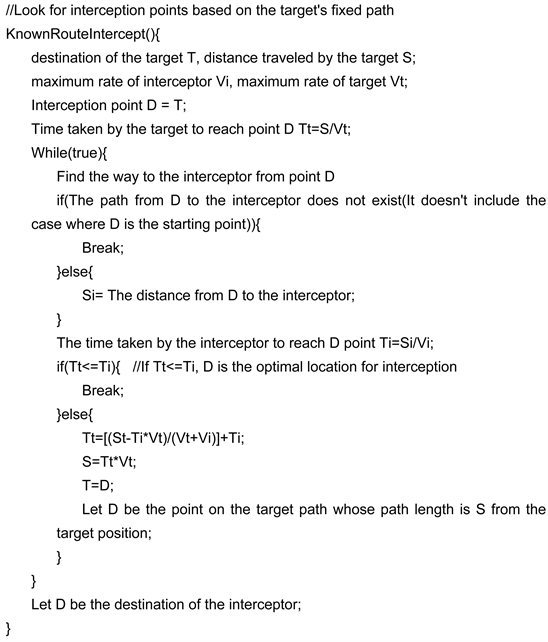
Of course, due to the needs of actual game applications, the time complexity of the algorithm should not be too high. The time complexity of this algorithm mainly lies in the loop call of pathfinding algorithm. In order to reduce the time cost, we can set a threshold value for the loop times to lessen the call times of pathfinding algorithm. In addition, in order to reflect the authenticity, we can set the algorithm only be used in the map which is known to the interceptor.
3.3.2. Real-Time Moving Target
For a moving target, we can regard it as the second or the third interception scenario in reality. The third case is special which is not applicable if there are many static obstacles in the map, so it can only be invoked when the distance between the interceptor and the target is close and the nearby obstacles are little. In other cases, the second interception scenario, call of the pathfinding algorithm, is used, which detects the location of the target at the next moment and sets it as the destination of interceptor.
In order to distinguish which scheme to use, we need to traverse the map in a certain range first, and then decide using which interception method according to the number or proportion of obstacles in the range. The traversal scope should at least include the target and interceptor, as well as computer performance. Here is a way to determine the scope. First, get a predicted node by multiplying velocity of the target by a certain time. The interceptor is then wired to the target and the predicted node respectively. Finally, a rhomboid formed by the two straight lines is used as the range. The problem here is to set a threshold for the number or proportion of obstacles.
The problem here is to set a threshold for the number or proportion of obstacles. If the value is set too large in the maze terrain, the predicted destination, interceptor, and target may not be in a connected graph, as shown in Figure 1.
This can cause the interceptor to move away from the target. Therefore, we need to judge whether the three are in the same connected component while scanning the disorder.
4. A* Pathfinding Algorithm and Its Improvement
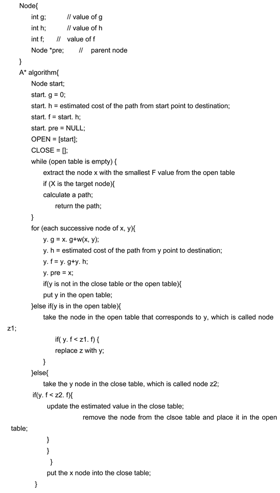
4.1. Introduction to A* Algorithm
Because the basic pathfinding algorithm of this scheme is A* algorithm, therefore, the general principle of it is briefly described here.
A* algorithm uses g(n) to represent the path cost from the starting point to any node n, and h(n) to represent the estimated cost (heuristic value)of the path from node n to the target node. Define the estimated value f(n) = g(n) + h(n), and the A* algorithm will detect each node with the minimum f(n) value. Select the path by maintaining Open table (for holding extendable nodes) and Closed table (for holding non-extendable nodes).
A* algorithm combines the advantages of Dijkstra algorithm and greedy algorithm, that is, it guarantees to find the shortest path and fast pathfinding speed.
![]()
Figure 1. The case where the interceptor, the target, and the predicted destination are not in the same connected component.
The pseudo-code is as follows:
4.2. Improvement of Obstacle Detection of A* Algorithm
In A* algorithm, obstacles are considered as non passable points and are not considered. However, there are many obstacles and terrain that can be passed through in a special way. Many games use collision detection to identify obstacles. If the three-dimensional space is taken into account, the obstacles in the two-dimensional plane can be divided into two categories. One kind of obstacle is called passable obstacle, which can pass through by special moving ways, such as the obstacle that can crawl through, the obstacle that can jump or fly through, and the obstacle that can pass by side. The other kind is impossible to pass through, such as the seamless wall directly connected with the ceiling and the ground. For accessible obstacles, an obstacle eigenvalue group can be added for obstacles (including units), which can be set according to actual needs. Then set the corresponding capacity value for the mobile unit. Finally, through the simple addition and subtraction calculation, the obstruction value is added to the g value of the corresponding grid. This improvement is relatively simple, so it will not be described in detail.
5. Improvement of A* Algorithm for Dynamic Obstacles
5.1. A* Algorithm Deals with Dynamic Obstacles
When there are multiple moving objects in the game map, each moving object may become an obstacle to other units, and such obstacles in movement are not under consideration of A* algorithm, so it is necessary to improve A* algorithm for dynamic obstacles.
In a map with multiple dynamic obstacles, the amount of computation, which required for taking the movement of all units into account to calculate the interceptor’s course of action, is incalculable and does not meet the game’s rapid feedback requirements. Therefore, a strategy of responding to the dynamic obstacles within the specified range or when the collision occurs is usually adopted.
There are generally two strategies for dynamic barriers: 1) Re-select the path, 2) Steer clear of obstacles.
For the first strategy, the two most common ways to re-select paths are path clipping and monitor map changes. Since the path after editing is likely to be no longer the optimal path and does not meet the interception requirements, this scheme mainly discusses the method of monitoring map changes, that is, triggering recalculation according to map changes. The map grid re-scants and records when it receives a terrain change or a collision between units.
However, when more than one unit moves or the map changes frequently and continuously, this method can lead to the need to recalculate at every moment, thus consuming a lot of time. Therefore, the original method is more suitable for the situation where the obstacle changes are less and not in a continuous state. This method needs to be improved for maps with persistent movement obstacles.
For the second clock strategy, the traditional algorithms to avoid collision, such as collision avoidance RVO (Reciprocal Velocity) or repulsive force, belong to the obstacle avoidance algorithm, that is, they return to the original path after detour when encountering Obstacles. When used in combination with A* algorithm, a better effect will be achieved if there are many and dense routes to the end point. However, in the case of few channels which are scattered, this scheme is prone to lead to long waiting, or unnecessary back and forth movement, as shown in Figure 2.
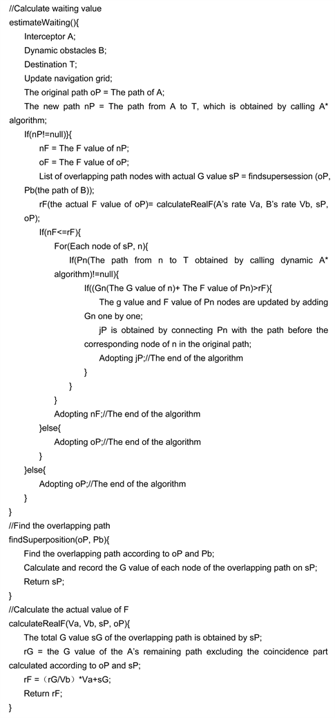
Combining the above two strategies, when the interceptor’s path is blocked by dynamic obstacles, the key to the problem is to determine the waiting value of the obstacles, so as to decide whether to find another way or to wait.
In this scheme, the obstacles are divided into the obstacles with instantaneous change (terrain transformation) and the obstacles with continuous change (moving unit). For the instantaneous change of obstacles, the method of monitoring map is adopted. For the continuous change obstacle, the algorithm is used to determine whether to change the path after calculating the wait value of the obstacle when the collision occurs. The latter algorithm is implemented as follows:
When a path is blocked or a collision occurs (the interceptor’s speed is greater than that of the moving obstacle), the interceptor restarts the pathfinding. If no path is available, wait to move (the so-called waiting movement, that is, when the front obstacle, according to the original path movement. And will no longer trigger collision determination). Otherwise, call out the original moving route of the interceptor and the blocking unit, and calculate the G value of the overlapping path of the two (since the path length can be obtained by multiplying the G value by the grid proportion, which has no real effect in the operation, so the G value can be used to directly replace the path length calculation). The G value of the overlapping path is divided by the obstacle movement rate to get the time that the interceptor actually passes the distance. Multiply the actual time times the maximum rate of the interceptor to get the actual value of G. The sum of the actual G value and the interceptor’s original path divided by the G value of the rest of the coincidence path is the actual F value of the original path. The formula is expressed as follows:
The G value of the overlapped path/the speed of the obstacle = the actual time taken.
The actual time taken * the interceptor’s rate = the actual value of G.
The actual value of G + the G value of the remaining path = the actual value of F.
![]()
Figure 2. Channel blockage caused by dynamic obstruction.
Compare the actual F value with the F value of the new route. If the F value of the new route is larger, the new route will be adopted; otherwise, the waiting movement will be carried out.
5.2. Waiting Valuation Algorithm
5.2.1. The Basic Idea of the Algorithm
The problem in this scheme is that there may only a small part of the overlap in the original path is necessary. In the rest, the interceptor can move around the dynamic barrier. Therefore, the path waiting for detour may be better than the newly found path. See Figure 3.
This leads to a new path that deviates from the algorithm’s goal of speeding the interceptor to the target location. Therefore, the possibility of detour must be taken into consideration to further optimize the algorithm.
First, the algorithm needs to know where the detour is likely to occur and how to determine the value of the detour.
When the interceptor and the moving obstacle move along the coincidence path, detour may occur if there are other passable grids in the interceptor’s grid. The detour is valuable when the actual F value at the end of the detour is smaller than the F value of the new path. Thus, the following algorithm schemes can be obtained:
Va (the maximum rate of A) > Vb (the maximum rate of B). Both Va and Vb are known. The path of A starting from its current position is set as Pa, while the path of B starting from its current position is set as Pb. When A and B collide or approach, the following processes are triggered:
1) Re-scan the navigation grid of the map and add B as an obstacle. Based on the new navigation grid, call A* algorithm for A to find the new path Pn to reach the original target point T of A. If there is no new path, the path will not change, and the wait move strategy will be adopted. Execute (2) if a path is found (of course, the connected graph can also be used to determine in advance whether there is a new path, so as to reduce the problem of high pathfinding time when there is no path. However, since this is not the core content of this algorithm, it will not be explained in detail.
![]()
Figure 3. Comparison between the ideal detour path and the path obtained by re-routing.
2) Fn is the F value of the new path obtained from A* algorithm. Then, according to Pn, Pa and the formula for calculating the actual F value mentioned above, the actual G value corresponding to each grid of overlapping grid Ps can be obtained, and the actual F value of the original path, F', can be calculated. If Fn ≤ F', execute (3). Otherwise, the path remains the same and the wait move strategy is adopted.
3) Starting from the grid of B, each overlapping grid G is scanned. If unit can move in another direction at G, then execute (4). Otherwise, look at the next grid until all the overlapping grids have been scanned once. If G is not met, Fn is adopted as the new path.
4) Calculate the path Po from G to the destination via the dynamic A* algorithm, which will be described below. To reduce the time complexity, the pathfinder can be narrowed. In addition, the point where A and B are located should be treated as an obstacle to prevent backward pathfinding so that the path found is the coincident with the path obtained from Pn connecting the overlapping path in front of G. The F value of the transcending route Po is added to the actual G value Gg corresponding to G to obtain the actual F value Fo' of the transcending route Po. The calculation method of the actual F value of all overlapping grids before St is as follows:
Let all the overlapping grids start from the grid of B and be marked as P0, P1, P2, ∙∙∙, Pt, ∙∙∙, Pn and their corresponding G values are G0, G1, G2, ∙∙∙, Gt, ∙∙∙, Gn, which have been obtained in (2). The Fs' of the next grid can easily obtained by adding the actual G value corresponding to the previous Fs'. The formula is as follows:
Judge whether Fo' < Fn is true. Because Fn ≤ F', the condition also shows that the transcendental path is better than the original path. If it is true, Po and Pt are spliced to obtain path P. After the g value of each node of Po segment in P is updated according to Gg, P is taken as a new path of a, and the waiting move strategy is adopted. The algorithm effect is shown in Figures 4-6.
![]()
Figure 4. The path obtained by using A* algorithm in the experiment.
![]()
Figure 5. The path obtained by the waiting valuation A* algorithm in the experiment.
![]()
Figure 6. The flow chart of the algorithm.
The pseudo-code of the process is as follows:
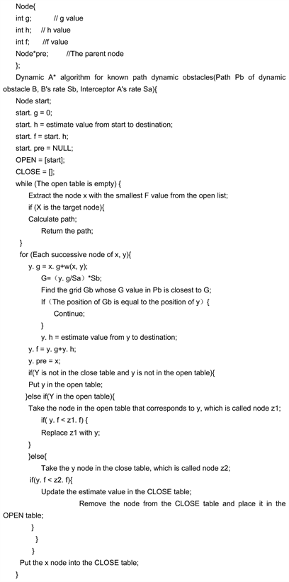
5.2.2. Dynamic A* Algorithm for Dynamic Obstacles with Known Paths
In order for the A* algorithm to adapt to known path dynamic obstacles, an improvement can be made in the ordinary A* algorithm to take the path of the dynamic obstacle into consideration. Specifically, each time when looking for the next node N, according to the G value of N Gn, Interceptor A’s speed Sa, dynamic obstacle B’s speed Sb and the G value Gb at the point where B is located can be calculated as (Gn/Sa) * Sb. If a node with a G value equal to Gb exists on the B path, and the position of the node coincides with N, N is treated as an obstacle.
The pseudo code is as follows:
5.2.3. Improvement for Time Complexity 1—Threshold
When using the method proposed above, the A* algorithm has to be called multiple times. This will greatly increase the time complexity of pathfinding and seriously affect the pathfinding effect and game experience. Therefore, we need strategies to reduce the computation time of the A* algorithm. In addition to the two strategies described above that use connected graphs to predict and narrow the path search range, the actual F-value introduced in the previous section can also be used as a threshold to limit the time-consuming time of the A* algorithm. In (4), St calculates Fs' before calling A* algorithm for path finding. In the process of path finding, when the F value of the node fetched from the open table plus Fs' is greater than Fn, then the path finding fails directly. The same applies in (1), and the threshold value should be set to F'.
5.2.4. Improvement for Time Complexity 2—The Maximum Number of Evaluation Grids
The above process is only evaluated once and is applicable to a smaller pathfinding range. For a wide range of pathfinding, without multiple wait valuation, it may still lead to a detour. Therefore, we can use it several times as long as the computing power permits, so as to make a waiting valuation for all the overlapping paths, and then compare to get the shortest route.
5.3. The Presentation of Waiting Valuation Algorithm
We implemented the algorithm in unity3d and carried out simulation experiments. As shown in Figure 7, we set two balls target to the black ball. The red one uses A* algorithm to find its path, and the blue one uses both waiting valuation algorithm and A* algorithm. The line composed of red squares represent the pathfinding results of blue ball by using waiting valuation algorithm, while the blue one is corresponding to A* algorithm. The data in the picture are the speed parameter and path-cost which is used to evaluate the time taken by certain path.
![]()
Figure 7. Comparison of the two algorithm paths.
It’s obviously that the waiting valuation algorithm can find the actual optimal path.
6. Concluding Remarks
Just like playing Go, it is immeasurable and unnecessary to spend a lot of time simulating all the solutions in a single calculation to find the optimal solution in the face of dynamic development. Therefore, by referring to the idea of divide and conquer, we can complete the whole process in stages, rather than in a single plan. For each step, we may analyze it as a dynamic programming problem. At this point, in solving the small dynamic programming problem, the algorithm can be used to realize the local optimal solution, so as to achieve certain predictability and intelligence. Each step of the interception problem can be divided into time slices.
When faced with a problem with multiple possibilities at one time, one of the core lies in making full use of known information to eliminate the unknown to reduce the scale of the problem. Based on this idea, this scheme proposes a known path interception algorithm, which solves the problem of AI facing complex terrain when intelligently intercepting game units. At the same time, on the basis of A* algorithm, an improved waiting valuation algorithm for dynamic obstacles is derived. Different from the traditional method, this algorithm combines the advantages of re-selecting the path and avoiding obstacles to bypass, so that the AI can decide to adopt different strategies and paths according to the actual situation, while also ensuring the optimization of the path.
Of course, there are still some problems with this scheme. Because the scheme is based on and repeatedly calls the A* algorithm, its time complexity is directly related to the time complexity of the A* algorithm and the number of calls. As the distance increases, so does the time and frequency of pathfinding, making it difficult to adapt to long-distance interception. In addition, the algorithm for judging whether a certain area map is a connected graph is not implemented in the solution, and this algorithm can greatly reduce the time consumption of this solution, and it is also the algorithm required for the special interception situation mentioned above.