Detecting Pipeline Anomalies and Variations in Acoustic Velocity in Multiphase Flow Regimes Using Computational Fluid Dynamics

Amod Kumar, Claudio Olmi, Oluwatosin Ogundare^*, Pranab Jha, David Bennett

Halliburton Energy Services Inc., Houston, TX, USA.

DOI: 10.4236/ojfd.2020.103012                

Abstract

The use of hydrodynamic pressure wave generated from the action of a fast acting valve as well as acoustic reflectometry in the detection of anomalies like leaks, deposits and blockages in a pipe or fluid flow system in the context of the prevailing scientific theories in fluid flow is discussed. The focus of this paper is the application of the theories to more complex scenarios involving multi-phase fluid flow, specifically, two-phase and two-component fluid flow. The principal concern is the determination of acoustic velocity in a two-phase flow regime; which is problematic because it varies with mixture composition along multiphase flowlines. A technique for simulating flow regimes in the laboratory using stacked S-shaped pipes is presented as well as a discussion of the results from a computational fluid dynamics model.

Keywords

Multiphase Flow, Acoustic Reflectometry, Pipeline Anomaly, Acoustic Velocity

1. Introduction

Deposit of wax and other scales in pipelines used for oil extraction and transportation is very common. Such scaling on the pipeline may lead to a significant pressure reduction in production or fluid carrying capacity of the pipelines. The standard method to locate the position and size of such deposits is based on reflection of waves due to changes in cross-section area where the wave itself is generated by the action of a fast acting valve. The closure of the valve generates a pressure wave known as water hammer, and the speed of propagation of the wave in the fluid media is a deciding factor on the accuracy of the subsequent analysis. In its simplest form, the speed of the pressure wave can be derived from the Joukowsky’s formula ∆P = [ρc∆V], where ΔP is the observed pressure spike; ρ is the density of the fluid; c is the average speed of sound in the fluid; and ΔV is the change in mean flow velocity. In the case of single-phase flows, the speed of sound can be estimated by correlations, which has good accuracy and covers all sorts of pipeline dimensions such as thickness and fixation. On the other hand, the speed of sound and flow pattern in two-phase flows related to oil and gas applications exhibit a lot of variation; therefore the extension of the single-phase flow to two-phase flow conditions for detection of deposits require special validation of flow regimes and calculation of speed of sound. Since two-phase flow conditions are widely encountered in the transportation of crude oil, a precise and accurate way of detecting deposition in two-phase flows will help the industry reduce turn-around time and save cost [1] - [6].

Much research has already been done pertaining to sound speed for single-phase flow and readers can refer to Chaudhry [4] for a detailed theoretical exposition of single-phase flow transient phenomenon. Most of the research in two-phase flow has been done using water as the fluid medium, given its availability as test medium and varied applications (pipelines, ocean flows, etc.). In the field of petroleum engineering, Wang et al. [7] have provided acoustic velocities in oil that are strong functions of pressure and temperature. Additionally, Wang et al. [8] provided empirical equations to calculate acoustic velocities in oils with known API gravities.

As indicated, there are several alternative methods to locate and quantify deposits or other anomalies in pipelines, but they all require expensive sensors and they mostly apply to non-buried pipes. Precise capture of location of the deposit is critical to plan the clean-up activities. A large variation in the predicted location of deposits may result in partial cleaning or no cleaning at all.

Another common anomaly in pipe systems is leakage. Leak detection in pressurized single-phase pipelines is a very well-studied problem. Various groups have contributed to the knowledge of using transient pressure pulses to detect leak location and quantification [9] [10] [11]. Similarly, methods for blockage or deposit detection [12] [13] [14] [15] and corrosion losses [16], [17] in pipelines and utility piping systems are well documented. For example, Lee et al. [18] used an impulse response function to find leaks in pipelines. They compared the transient behavior of a leaking pipe with that of a non-leaking one.

In multiphase flows, the propagation of pressure pulse in two-phase mixtures has been studied extensively in the context of nuclear engineering and phase changing fluids [19] [20]. In oil and gas, Gudmundsson and Celius [21], utilized pressure pulse to calculate the mass flow rate downhole, at the wellhead and proposed a multiphase metering method. Acoustic reflectometry for blockage detection has also been explored recently [13] [22] [23].

2. Materials and Methods

2.1. Calculating the Speed of Sound in Homogeneous Isotropic Media

As evident in the Joukowsky’s equation, the critical components in estimating the pressure rise due to a transient event are density, sound speed and change in velocity. The governing equations for wave propagation in a pipe flow are a set of hyperbolic partial differential equations, given below.

$\frac{\partial U}{\partial t}+B\frac{\partial U}{\partial x}=E$ (1a)

where

$U=\left(\begin{array}{c}p\\ V\end{array}\right)$ (1b)

$B=\left[\begin{array}{cc}V& \rho c^2\\ \frac{1}{\rho }& V\end{array}\right]$ (1c)

$E=\left(\begin{array}{c}0\\ -g\sin \theta -\frac{fV\left|V\right|}{D}\end{array}\right)$ (1d)

The eigenvalue of matrix B can be deduced as $\lambda =V\pm a$.

Fluid velocity is generally known in a pipeline transporting oil and gas mixture. Assuming, a one-dimensional (1D) problem, the density of a fluid can be estimated using various available models; therefore, the sound speed in conduits is easy to estimate for single-phase liquid flows. The speed of a wave travelling in an elastic pipe with homogeneous isotropic media can be computed using parameters from the media and the pipe characteristics as found in literature [5], [24]. The formula is

$c=\sqrt{\frac{1}{\rho \left[\frac{1}{K}+\frac{D\psi }{E\epsilon }\right]}}$, (1e)

where $\rho ,K$ are respectively the density and stiffness (or bulk modulus) of the media, and $E,\epsilon ,\psi ,D$ are respectively the Modulus of Elasticity, thickness, support factor, and diagonal dimension of the pipe. The pipe support factor can be ignored, $\psi =1$, when $D/\epsilon >10$ and bulk modulus is large.

In terms of oil and gas pipeline, it is relatively easy to estimate the wave speed for a homogeneous fluid or gas [6]. On the other hand, it is tedious to provide a calculated speed of sound for multi-phase fluids that include an often-unknown distribution of the percentage mixture of gases, liquids, and solids. Compounding to the mixture variability issue, there is no assurance that the mixture is constant for the whole length of the pipe.

Furthermore, acoustic velocity is directly influenced by the frequency content of the wave if there is dispersion. Pulse waves contain a theoretical infinite frequency band, but real water hammers are subjected to band limitations imposed by the valve characteristics.

2.2. Measuring Speed of Sound in Homogenous Isotropic Media

When a wave is generated from one end of a pipe, the wave front will travel to the other end in Δt time, also called the communication time. The relationship between the speed of sound and the communication time is given by

$c=\frac{2L}{\Delta t}$ (2)

where c is the wave speed and L is the length of the pipe. Thus, by inducing a pressure wave pulse at one end of the pipe, we can measure when the reflected wave comes back to the source, and then calculate the average speed of sound for any media. Measuring the value of acoustic velocity is not successful if dealing with multi-phase fluids.

If the transmitted signal is set to individual sine waves, we can measure the speed of sound in the media for the selected frequencies (or a Bode plot with dB attenuations). For non-dispersive medium, the speed of sound is independent of wave frequency and we would just see a flat horizontal line. In the other case, we will have a curve that identifies the frequency with the maximum and minimum speed of sound and attenuation.

2.3. Attenuation of Pressure Waves in Homogeneous Media

While the acoustic waves move along the pipe length, the fluid itself introduces attenuations. It is typically calculated as follows:

$P=P_s{\text{e}}^{-\alpha z}$ (3)

where $P_s$ is the acoustic pressure wave in Pascal, $\alpha$ is the attenuation factor, and z is the distance from the acoustic source. The attenuation factor is related to the fluid characteristics as follows:

$\alpha \left(\omega \right)=\frac{\left(2\eta +\frac{3}{2}{\eta }_v\right)\omega }{3\rho c_{\omega }}$ (4)

where $\eta$ and ${\eta }_v$ is the dynamic and volume viscosities of the fluid, $\rho$ is the density of the fluid, and $c_{\omega }$ is the speed of sound for the specific angular frequency.

2.4. Dispersion in Anisotropic Media

When dispersion occurs, it affects individual frequency components of a pulse wave travelling in a pipeline. This is where we need to redefine the speed of sound as a function of frequency. The phase velocity $c_p$ changes depending on the frequency. The speed of sound tables found in books only reports group velocities $c_g$ of common media, and they represent the highest speed $c_g={\max }_f{c}_p$. The group velocity is calculated by considering the ratio of axial to angular wavenumber for the specific mode as thus:

$c_{g,m}=\frac{{\kappa }_m}{K_m}{c}_p$ (5)

In general the dispersion equation relates the wavenumbers to each other as $k^2={\gamma }^2+{\kappa }^2$.

2.5. Wave Reflection and Refraction Due to Impedance Changes—Snell’s Law

When a wave crosses the interface of two isotropic media, there is a change in impedance, the wave gets refracted and/or reflected depending on the angle of the incident wave following Snell’s law, which tells us that the incident crossing wave i, has a change in impedance at an angle θ_i with wave speed c_i will be refracted into the new impedance at an angle θ_r and with wave speed c_r. Depending on the impedance and angle, the refracted wave will have a longitudinal and/or shear component with subscript l and s. In fluids, the shear component is not present.

2.5.1. Maximum Frequency

Since only plane waves propagate in long pipes, for a pipe to act as a waveguide, the pipe diameter must be such that the diameter, D is realized as follows:

$D<\frac{0.586c}{f_{\max }}$ (6)

where c is the speed of sound in the fluid and $f_{\max }$ is the maximum wave frequency. This formula only works for round pipes.

2.5.2. Measuring Attenuation across a Frequency Spectrum

Measure two or more points and verify that the cross-correlation among them shows that the sensors are reading the same signal. Also by computing the Power Spectral Density (PSD) of both signals in dB, we can then get the attenuation in dB divided by the distance between sensors.

$a\left(f\right)=\frac{d{B}_t\left(f\right)-d{B}_r\left(f\right)}{2L}$ (7)

2.6. Characteristics of Multiphase Flow Regime

2.6.1. Stratified (Smooth and Wavy) Flow

Stratified flow consists of two superposed layers of gas and liquid, formed by segregation of gas under the influence of gravity and buoyancy.

2.6.2. Intermittent (Slug and Elongated Bubble) Flow

The intermittent flow regime is usually divided into two sub-regimes:

· Slug flow—the gas is in the form of large bullet-shaped bubbles separated by slugs of coninuous liquid that bridge the pipe and contain small gas bubbles.

· Plug or elongated bubble flow—this flow regime can be considered as a limiting case of slug flow, where the liquid slug is free of entrained gas bubble. Gas-liquid intermittent flow exists in the whole range of pipe inclinations and over a wide range of gas and liquid flow rates.

2.6.3. Annular-Mist Flow

During annular flow, the liquid phase flows largely as an annular film on the wall with gas flowing as a central core. Some of the liquid is entrained as droplets in this gas core (mist flow).

2.6.4. Dispersed Bubble Flow

At high liquid rates and low gas rates, the gas is dispersed as bubbles in a continuous liquid phase. The bubble density is higher toward the top of the pipeline, but there are bubbles throughout the cross section. Dispersed flow occurs only at high flow rates and high pressure and entails high-pressure loss.

For flows in horizontal pipes, various flow maps have been developed based on experimental observations, Baker’s map and Taitel-Duckler maps (as shown in Figure 1) being prominent among all maps. The two maps differ in the variables chosen to define the boundaries of flow pattern and typically both maps yield similar results.

Figure 1. Flow map—Taitel and Dukler for horizontal pipes [25].

The foundational equations relating to flow regimes in multiphase flow are stated as follows:

$F=\sqrt{\frac{{\rho }_G}{{\rho }_L-{\rho }_G}\frac{v_{SG}}{\sqrt{dg\cos \theta }}}$ (8)

$K=F\sqrt{R{e}_{SL}}$ (9)

$T={\left[\frac{-\frac{\text{d}p}{\text{d}L}}{\left({\rho }_L-{\rho }_G\right)g\cos \theta }\right]}^{0.5}$ (10)

The subscripts G and L refer to the gas and liquid phases respectively. The subscript SL stands for “superficial liquid”, the velocity and Reynolds number resulted by assuming only liquid flowing through the pipe. F is used to check for stratified to non-stratified transition, T is used to check for stratified-smooth to stratified-wavy transition.

For a reliable production model, finite element analysis has to be employed to solve for the acoustic velocity in the multiphase mixture. Theoretically, the acoustic velocity may vary in different pipe grids or slices. Several experimental datasets have been reported in literature, which provides the speed of pressure waves in a gas-liquid mixture. Brennen (Brennen, 2005) illustrates this fact using data from several sources. The speed of sound in a bubbly mixture can be much smaller than either in liquid or gas, as shown in Figure 2. This basic difference exists due to the density difference between the phases. In most analyses, the surface tension effects can be neglected under the assumption that the gas bubbles have the same pressure as the fluid outside it. This leads us to an adiabatic system, wherein, the speed of sound is slightly different when compared to an isothermal system, as illustrated in the figure. Of course, the gas constant, k, usually takes into account this fact. The mixture acoustic velocity for a particular pipe slice or grid can be calculated using the following simplified equation:

Figure 2. Expected change in acoustic velocity with volume fraction of gas.

$\frac{1}{c_{TP}^2}=\frac{\alpha }{kp}\left[{\rho }_L\left(1-\alpha \right)+{\rho }_G\alpha \right]$ (11)

Wood’s low-frequency speed of sound or the Wood limit of the speed of sound in bubbly liquid plotted in the above chart is expressed by following correlation where α is the volume fraction of the gas, subscript TP represents two-phase conditions and c is speed of sound (the wave speed).

$\frac{1}{c_{TP}^2}=\frac{{\alpha }^2}{c_G^2}+\frac{{\left(1-\alpha \right)}^2}{c_L^2}+\alpha \left(1-\alpha \right)\times \frac{{\rho }_G^2{c}_G^2+{\rho }_L^2{c}_L^2}{{\rho }_L{\rho }_G{c}_L^2{c}_G^2}$ (12)

The overall acoustic velocity, for practical considerations is the harmonic mean of the mixture acoustic velocities in the different pipe grids or slices (assuming the grids have a constant cross-sectional area).

2.7. Set-Up for Flow Regime Generation and Acoustic Velocity Measurement in the Laboratory

Figure 3 shows the experimental set-up for the generation of different flow regimes to verify its impact on acoustic velocity and its dependence on gas fraction, and liquid flow rate.

The goal of the test is to validate the flow regimes (two-phase flow patterns such as stratified or slug or plug flow) and measure speed of propagation of pressure wave under these conditions.

Figure 3. Test set-up for two-phase flow measurements.

A simple and fast two-dimension simulation was conducted to verify that the pressure transient predicted by the CFD simulation software matched empirical correlation presented as Joukowsky’s formula.

3. Results

The example case in this study is a system for inducing multiple flow regime in a 2-phase, 2-component flow using connected stacked horizontal pipes: The new method extends principles used in single-phase applications to two-phase conditions. Based on empirical correlations and expected gas-liquid volume fraction in the oil and gas industry, the flow rates for gas (air or nitrogen) and water are estimated.

Flow regimes in horizontal pipes selected for investigation as per Baker’s map in Figure 4, are summarized in Table 1 and Table 2.

Since the liquid and gas under investigation are water and air respectively, λ and ψ equal 1 for this application. The gas volume fractions for the 6 operating points identified in the above plot are summarized in the following table. The mean operating pressure of 1.013 [bar] absolute and temperature 25 [˚C] was considered. The calculation was performed for a 2 [in] diameter pipe and the superficial gas and water velocities may change based on the cross-section area

Table 1. Description of realized flow regimes in connected stacked horizontal pipes of inner diameter 2.

Table 2. Description of realized flow regimes in connected stacked horizontal pipes (Cont.).

Figure 4. Bakers map and associated equations [26].

of the pipe. The estimated superficial velocities of gas and liquid also denote the slip one can observe between the two phases.

3.1. Verification of Pressure Transient Simulation in Single Phase

A CFD simulation in two-dimension axisymmetric domain was carried outto check the simulation setting and accuracy of results to predict pressure rise during water hammer phenomena. The simulations were initially done in single phase and subsequently extended to multi-phase with air volume fractions at 1% and 5%.

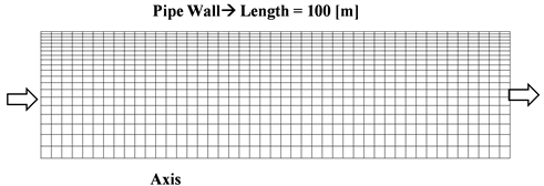
Step-1: Prepare an axisymmetric computational domain with 100 [m] in length and 0.9718 [m] in diameter.

Step-2: Calculate the steady state flow simulation with “total pressure” at inlet and “static pressure” at outlet boundaries. Adjust the inlet pressure till a velocity of 1 [m/s] is achieved at the inlet.

Step-3: Once the steady state flow develops in the pipe, change the simulation to transient conditions and change outlet boundary conditions to the type “wall”. This represents sudden (instantaneous) closure of the valve. Solve the transient wave propagation for 3 - 4 cycles as estimated in Table 3.

As evident from the values of water hammer head calculated based on Joukowsky’s formula and CFD result, a close agreement between the peak pressure values was obtained as shown in Figure 5.

Table 3. System verification parameters for multiphase flow in reference pipe system.

Figure 5. Water hammer from Joukowsky’s equation.

Step-4: Repeat the process for two-phase flow conditions

Multi-phase flow simulation using mixture model and Eulerian model were carried out with 5% volume fraction of air in the air-water mixture flow in a pipe of diameter 100 [mm].

Since the CFD simulation approach does not resolve the compressibility effect of air on the mixture and subsequent wave propagation, the impact of air present in the flow stream was not observed on the water hammer value estimated in the simulation. At 5% volume fraction, the speed of sound in water-air mixture is measured around 1000 [m/s] which is consistent with Figure 2.

Table 4. Compressible-liquid setting in ANSYS FLUENT.

Figure 6. Eulerian model—inlet boundary—volume fraction of air and water.

Hence, in case one needs to use CFD methods to simulate water hammer conditions, the reference bulk modulus needs to be appropriately adjusted to match the desired wave speed. The reference values are shown in Table 4.

3.2. Simulation Results for 1% Volume Fraction of Air

The purpose of this multi-phase flow simulation was to check the effect of gas content on pressure drop per unit length of pipelines and test the accuracy of CFD simulation methods for such cases. A mixture model with realizable k-α turbulence model was used in ANSYS FLUENT. Simple method for pressure-velocity coupling and second order discretization scheme for momentum equation was used. A good convergence of residuals was obtained.

At low volume fraction of gas, the mixture model predicts air as small bubbles dispersed in continuous phase. Figure 6 shows Eulerian model for the simulation done with 1% gas fraction.

4. Conclusion

The pressure drop value reported in the CFD simulation is 5020 [Pa] which is expectedly lower when compared to single phase flow pressure drop of 5498 [Pa] estimated as per Haaland’s equation. After initial validation of the CFD simulations for single phase and two-phase flow conditions, we determined that the simulation approach benefited from adjustments or refinements made for practical considerations. The authors find that the laboratory set-up presented prior is sufficient to replicate the two-phase behaviors namely plug, stratified, slug, wavy, annular and bubbly flow regimes and that any inherent uncertainties associated with two-phase flow maps such as Baker’s map can be mitigated as a strong function of differential pressure and gas fraction based on the observations.

Conflicts of Interest

The authors declare no conflicts of interest regarding the publication of this paper.

References

[1]	Mellor, D.W. and Millar, J.W. (1992) U.S. Patent No. 5,170,378. U.S. Patent and Trademark Office, Washington DC.
[2]	Chin, W.C. and Trevino, J.A. (1988) U.S. Patent No. 4,785,300. U.S. Patent and Trademark Office, Washington DC.
[3]	Rostron, P. (2018) Critical Review of Pipeline Scale Measurement Technologies. Indian Journal of Science and Technology, 11, 1-18. https://doi.org/10.17485/ijst/2018/v11i17/121459
[4]	Chaudhry, M.H. (2014) Applied Hydraulic Transients. Springer, New York. https://doi.org/10.1007/978-1-4614-8538-4
[5]	Gudmundsson, J.S. (2006) U.S. Patent No. 6,993,963. U.S. Patent and Trademark Office, Washington DC.
[6]	Hunaidi, O., Bracken, M. and Wang, A. (2008) U.S. Patent No. 7,328,618. U.S. Patent and Trademark Office, Washington DC.
[7]	Wang, Z. and Nur, A. (1991) Ultrasonic Velocities in Pure Hydrocarbons and Mixtures. The Journal of the Acoustical Society of America, 89, 2725-2730. https://doi.org/10.1121/1.400711
[8]	Wang, Z., Nur, A.M. and Batzle, M.L. (1988) Acoustic Velocities in Petroleum Oils. Journal of Petroleum Technology, 42, 192-200. https://doi.org/10.2118/18163-PA
[9]	Lee, P.J., Lambert, M.F., Simpson, A.R., Vítkovsky, J.P. and Misiunas, D. (2007) Leak Location in Single Pipelines Using Transient Reflections. Australasian Journal of Water Resources, 11, 53-65. https://doi.org/10.1080/13241583.2007.11465311
[10]	Lee, P.J., Vítkovsky, J.P., Lambert, M.F., Simpson, A.R. and Liggett, J.A. (2005) Leak Location Using the Pattern of the Frequency Response Diagram in Pipelines: A Numerical Study. Journal of Sound and Vibration, 284, 1051-1073. https://doi.org/10.1016/j.jsv.2004.07.023
[11]	Brunone, B., Ferrante, M., Covas, D., Ramos, H. and De Almeida, A.B. (2004) Detecting Leaks in Pressurised Pipes by Means of Transients. Journal of Hydraulic Research, 42, 105-109. https://doi.org/10.1080/00221686.2004.9641189
[12]	Mei, I.L.S., Ismail, I., Shafquet, A. and Abdullah, B. (2015) Real-Time Monitoring and Measurement of Wax Deposition in Pipelines via Non-Invasive Electrical Capacitance Tomography. Measurement Science and Technology, 27, 25403. https://doi.org/10.1088/0957-0233/27/2/025403
[13]	Vidal, J.L.A., Silva, L.L., Monteiro, P.C.C. and Netto, T.A. (2013) Acoustic Reflectometry for Blockages Detection in Pipeline. Proceedings of the Annual Offshore Technology Conference, Vol. 1, 213-221. https://doi.org/10.4043/24294-MS
[14]	Duan, H.F., Lee, P.J., Ghidaoui, M.S. and Tung, Y.K. (2011) Extended Blockage Detection in Pipelines by Using the System Frequency Response Analysis. Journal of Water Resources Planning and Management, 138, 55-62. https://doi.org/10.1061/(ASCE)WR.1943-5452.0000145
[15]	Wang, X.J., Lambert, M.F. and Simpson, A.R. (2004) Detection and Location of a Partial Blockage in Pipeline Systems Using Damping of Fluid Transients. Proc. 2004 World Water Environmetal Resour. Congr. Crit. Transitions Water EnvironmetalResour. Manag., Vol. 131, 4789-4798. https://doi.org/10.1061/40737(2004)475
[16]	Xu, Y., Huang, Y., Wang, X. and Lin, X. (2016) Experimental Study on Pipeline Internal Corrosion Based on a New Kind of Electrical Resistance Sensor. Sensors and Actuators B: Chemical, 224, 37-47. https://doi.org/10.1016/j.snb.2015.10.030
[17]	Xu, Y.Z., Yang, L.J., He, L.M., Huang, Y. and Wang, X.N. (2016) The Monitoring of Galvanic Corrosion Behaviour Caused by Mineral Deposit in Pipeline Working Conditions Using Ring Form Electronic Resistance Sensor System. Corrosion Engineering, Science and Technology, 51, 606-620. https://doi.org/10.1080/1478422X.2016.1173313
[18]	Lee, P.J., Vítkovsky, J.P., Lambert, M.F., Simpson, A.R. and Liggett, J. (2007) Leak Location in Pipelines Using the Impulse Response Function. Journal of Hydraulic Research, 45, 643-652. https://doi.org/10.1080/00221686.2007.9521800
[19]	Henry, R.E., Grolmes, M.A. and Fauske, H. (1971) Pressure-Pulse Propagation in Two-Phase One- and Two-Component Mixtures. Argonne, IL (United States). https://doi.org/10.2172/4043485
[20]	Hsu, Y.-Y. (1972) Review of Critical Flow Rate, Propagation of Pressure Pulse, and Sonic Velocity in Two-Phase Media. NASA Tech Note, Vol. TN D-6814, No. June, 1-45.
[21]	Gudmundsson, J.S. and Celius, H.K. (1999) Gas-Liquid Metering Using Pressure-Pulse Technology. SPE Annual Technical Conference and Exhibition, Vol. 1. https://doi.org/10.2118/56584-MS
[22]	Chen, X., Tsang, Y., Zhang, H.-Q. and Chen, T.X. (2007) Pressure-Wave Propagation Technique for Blockage Detection in Subsea Flowlines. SPE Annual Technical Conference and Exhibition, Anaheim, 11-14 November, 233-254. https://doi.org/10.2118/110570-MS
[23]	Papadopoulou, K.A., et al. (2008) An Evaluation of Acoustic Reflectometry for Leakage and Blockage Detection. Proceedings of the Institution of Mechanical Engineers, Part C, 222, 959-966. https://doi.org/10.1243/09544062JMES873
[24]	Halliwell, A.R. (1963) Velocity of a Waterhammer Wave in an Elastic Pipe. Journal of the Hydraulics Division, 89, 1-21.
[25]	Taitel, Y. and Dukler, A.E. (1976) A Model for Predicting Flow Regime Horizontal and near Horizontal Transitions Horizontal Gas-Liquid Flow. AlChE Journal, 22, 47-55. https://doi.org/10.1002/aic.690220105
[26]	Baker, O. (1954) Simultaneous Flow of Oil and Gas. Oil and Gas Journal, 53, 185-195.