A Comparative Study of Initial Basic Feasible Solution by a Least Cost Mean Method (LCMM) of Transportation Problem

Md. Munir Hossain¹, Mollah Mesbahuddin Ahmed²

¹Department of Mathematics, Bangladesh Military Academy, Chattogram, Bangladesh.
²Birshreshtha Noor Mohammad Public College, Dhaka, Bangladesh.

DOI: 10.4236/ajor.2020.104008                

Abstract

Transportation Problems (TP), as is known, are a basic network problem which can be formulated as a Linear Programming Problem (LPP). Transportation networks are built up in order to save transportation cost. In the solution procedure of a TP, finding an Initial Basic Feasible Solution (IBFS) is necessary to obtain the optimal solution. Optimality gives us the optimal route that prompts either most extreme benefit or least aggregate cost whichever is required. In this research paper, a new method named Least Cost Mean Method is proposed to obtain a better IBFS where row penalty and column penalty is brought out by the mean of lowest and next lowest cost of each row and each column of the cost matrix. The method is illustrated with numerical examples. To verify the performance of the proposed method, a comparative study is also carried out and observed that it is computationally easier and yielding comparatively better solution.

Keywords

Initial Basic Feasible Solution, Optimum Solution, Penalty Cost

1. Introduction

Special type of linear programming problem is known as Transportation Problem (TP). TPs predominantly discuss the distribution plan of a product from a number of sources (e.g. factories) to a number of destinations (e.g. ware houses). When addressing a TP, the practitioner usually has a number of origins and a number of destinations. The origin of a TP is the place from which shipments are dispatched. The destination of a TP is the place to which shipments are transported. In each origin a certain amount of a particular consignment is available. Similarly, each destination has a certain requirement. Transporting one unit of the consignment from an origin to a destination is known as unit transportation cost. The TP indicates the amount of consignment to be transported from various origins to different destinations so that the total transportation cost is minimized without violating the availability constraints and the requirement constraints.

The first systematic procedure in solving the TP was developed by F.L. Hitchcock [1] in 1941 and referred as Least Cost Method (LCM), which consists in allocating as much as possible in the lowest cost cell of the TP in making allocation in every stage. Then the North West Corner Method (NWCM) by Charnes et al. [2] which started with allocating at the upper left corner cell or the north-west corner cell. It is based on position but not on transportation cost. Hence this method usually yields a higher cost, which is much more than optimal cost. Since LCM is based on cost cells therefore it usually gives better result than NWCM.

Reinfeld and Vogel [3] introduced Vogel’s Approximation Method (VAM) which is the conventional method that gives better IBFS than LCM and NWCM. This method was developed by describing penalty as the difference of lowest and next to lowest cost in each row and column of transportation table (TT) and allocate to the lowest cost cell corresponding to the highest penalty. Kasana and Kumar [4] bring in Extreme Difference Method (EDM) calculating the penalty by taking the differences of the highest cost and lowest cost in each row and each column where allocation procedure is as similar as VAM. Aminur Rahman Khan [6] presented HCDM by defining pointer cost as the difference of highest and next to highest cost in each row and column of a transportation table and allocate to the minimum cost cell corresponding to the highest three pointer cost. Mollah Mesbahuddin Ahmed et al. [7] applied the first allocation on lowest odd valued cost cell and proposed to form an allocation table (ATM) to allocate rest of the allocation for finding an IBFS.

Priyanka and Sushma [5] developed Average Transportation Cost Method (ATCM) by describing penalty as the average of the costs in each row and column of TT and allocation is to be done in the lowest cost cell corresponding to the highest penalty. Priyanka and Sushma [9] introduced modified ATCM by finding penalty which is equal to the average of minimum two costs in each row and column. Kirca and Satir [10] developed a heuristic to obtain efficient IBFS called Total Opportunity Cost Matrix (TOCM) by adding row opportunity cost and column opportunity cost. Here row opportunity cost is the deduction between lowest cost and all other cost elements of that particular row. Using this TOCM Kalam and Bellel [8] presented a method where penalties are the average of the row opportunity cost (row penalty) and the average of the column opportunity cost (column penalty). Similarly column opportunity cost is the deduction between lowest cost and all other cost elements of that column. Recently Hossain et al. [11] have used TOCM and defined the penalty cost as the difference between the highest and the lowest cell in the respective row and column of the TOCM. Then allocate to the minimum cost cell corresponding to the highest penalty cost where computing penalty cost for each and every allocation is avoided to ease up the computational complication.

In this research, we studied TPs and its solution technique in details. We also studied various methods for finding an IBFS for TPs and observed that there is no unique method which can be claimed as the best method for finding an IBFS. Again there is no standard procedure by which we can measure the quality of a solution technique. We also observed that some of the methods are yielding optimal or near to optimal, but the computational procedure is time consuming and complicated. In this study we try to bring some change in the solution technique of the existing methods with an aim to make the solution technique computationally easier. In this proposed method we need to compute penalty cost only for the first allocation and rest of the allocations is determined by alternative allocation procedure. We also solve several numbers of numerical problems using existing method and proposed method.

2. Transportation Model

The general form of the TP is presented by the following Figure 1.

To describe the above transportation model following representations are to be used:

$O_i$ —Total number of sources, $i=1,2,3,\cdots ,m$

—Total number of destinations, $j=1,2,3,\cdots ,n$

$s_i$ —Amount of supply at source i

$d_j$ —Amount of demand at destination j

$c_{ij}$ —Unit transportation cost from source i to destination j

$x_{ij}$ —Amount to be transported from source i to destination j

The main purpose of the model is to obtain the unknowns’ $x_{ij}$ that will minimize the total transportation cost by satisfying the supply and demand constraints. Considering this objective TP can be formulated as follows:

Minimize: $z={\displaystyle \underset{i=1}{\overset{m}{\sum }}{\displaystyle \underset{j=1}{\overset{n}{\sum }}{c}_{ij}{x}_{ij}}}$

Figure 1. Transportation problem scheme.

Subject to:; $i=1,2,\cdots ,m$

${\displaystyle \underset{i=1}{\overset{m}{\sum }}{x}_{ij}\ge d_j}$ ; $j=1,2,\cdots ,n$

$x_{ij}\ge 0$ for all i and j

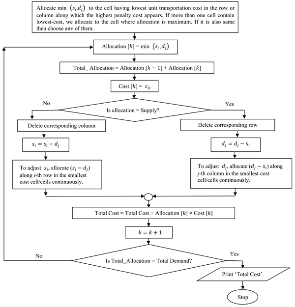
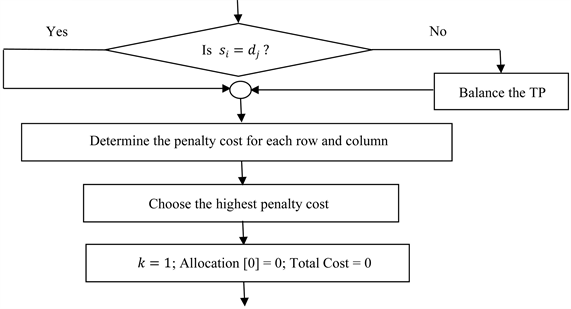
3. Algorithm

Step 1. Formulate the problem mathematically and if either (total supply > total demand) or (total supply < total demand), balance the given TP.

Step 2. Determine the penalty cost for each row by taking average of the lowest cell cost and the next lowest cell cost in the same row and put it on the right of the corresponding rows of the cost matrix. Similarly, calculate the penalty for each of the columns and write them in the bottom of the cost matrix below corresponding columns.

Step 3. Choose the highest penalty costs and observe the row or column along which it appears. If a tie occurs, choose the row/column along which lowest-cost appears.

Step 4. Allocate min $\left(s_i,d_j\right)$ to the cell having lowest unit transportation cost in the row or column along which the highest penalty cost appears. If more than one cell contain lowest-cost, we allocate to the cell where allocation is maximum. If it is also same then choose any of them.

Step 5. If the allocation $X_{ij}=s_i$, i-th row is to be crossed out and $d_j$ is reduced to $\left(d_j-s_i\right)$. Now complete the allocation along j-th column by making the allocation/allocations in the smallest cost cell/cells continuously. Consider that, j-th column is exhausted for the allocation $X_{kj}$ at the cell (k, j). Now, follow the same procedure to complete the allocation along k-th row and continue this process until entire rows and columns are exhausted. Again if the allocation $X_{ij}=d_j$, just reverse the process for $X_{ij}=s_i$.

Step 6. If the allocation $X_{ij}=s_i=d_j$, find the next smallest cost cell (i, k) from the rest of the cost cells along i-th row and j-th column. Assign a zero in the cell (i, k) and cross out i-th row and j-th column. After that complete the allocation along k-th row/column following the process described in step 5 to complete the allocations.

Step 7. Finally calculate the total transportation cost which is the sum of the product of cost and corresponding allocated value.

Flow Chart

4. Novelty of Our Algorithm

We work on exiting average cost method [5] [8] [9] and observe that computing penalty cost for each and every allocation is a computationally complicated and time consuming procedure. Therefore we try to avoid computing penalty cost for each and every allocation with a view to simplify the solution technique.

5. Numerical Example with Illustration

Example 1

Three fertilizer factories $O_1,O_2$ and $O_3$ are located at different places of the country produce 20, 28 and 17 lakhs tons of urea respectively. They are to be distributed to four district $D_1,D_2,D_3$ and $D_4$ as 15, 19, 13 and 18 lakhs tons respectively. The transportation cost per ton of fertilizer is given in the transportation Table 1:

Initial basic feasible solution using proposed method is given below (Table 2):

· According to Step 1 it is found that the given problem is balanced.

· According to Step 2 row penalty and column penalty is determined by the average of lowest and next lowest cost those are put on the right and bottom of the corresponding row and column respectively.

· Here in both 3^rd row penalty and 4^th column penalty is same i.e. 5. Since tie is occurred, therefore along those row and column lowest-cost appears in cell where the allocation is. With this allocation column is crossed out and supply along row is reduced to .

· As per Step 5 to complete the allocation of row, our next smallest cost cell along the row is cell. Now allocate remaining at the cell and cross out the row. After this allocation, demand along the column reduced to. In the column, the smallest cost cell where we put remaining as a next allocation and cross out column. Supply along the row reduced to.

Table 1. The given problem of example 1.

Table 2. Initial basic feasible solution obtained by LCMM.

· Now complete the allocation along row by making the allocation in the smallest cost (5) in the cell. Here row is exhausted for the allocation remaining units at the cell.

· In this stage, the allocation along column will be in the smallest cost (5) which is at the cell. By making the allocation of remaining units in the cell, the column is crossed out but the row is yet to exhaust. Then we will go for next smallest cost (1) along the row in the cell. Therefore row and column are exhausted simultaneously for the allocation remaining units at the cell.

· As per Step 7, total transportation cost is,

$11\times 3+9\times 5+19\times 1+9\times 5+4\times 7+13\times 3=209$

6. Numerical Example

We solve other three problems those have taken from some reputed journals. These problems along with their IBFS obtained by LCMM are tabulated in the following Table 3.

7. Result Comparison

We study the IBFS obtained by various methods. We carry out a comparative study of IBFS between proposed method and existing methods. To justify the perfectness of the proposed method a comparison is shown in the following table and chart (Table 4).

Table 4 represents the IBFS obtained by various methods, percentage of deviance from optimal solution and also the perfectness of the result in relation to

Table 3. Sampled data with corresponding IBFS and total cost using LCMM.

optimal result. It is observed that LCM and ATCM is numerically 25% and 75% cases equal to optimal result respectively. But our proposed method is 100% numerically equal to optimal result and NWCM performs nil in this case. This data analysis states the better performance of the proposed method. The following graphical representation of IBFS is also the reflect of this performance (Figure 2).

In Table 4, percentage of deviance from optimal result is obtained by the

formula $P_D=\frac{B_S-O_R}{O_R}\times 100$. This calculation is carried out to assess that how

much nearer the $B_S$ is to $O_R$. During this calculation it is observed that proposed method is near to optimal solution than the other methods discussed in Table 4. The percentage of deviance is shown in Figure 3.

Table 4. A Comparative study of IBFS.

*EO_R = Equal to Optimal, NO_R = Near to Optimal.

Figure 2. Graphical representation of IBFS.

Figure 3. Graphical representation of percentage of deviance.

8. Conclusions

Transportation cost is a significant part of a company’s overall logistic expenditure. The efficient and capacity of transport models has a direct impact on transport costs. To reduce the overall expenditure of any company, we need to provide a powerful framework to purchase and bring raw materials or it is to distribute finished goods with minimum transportation cost. In this study, we

propose a method LCMM to obtain an IBFS for the minimization of transportation cost. We illustrate the proposed method and solve few problems. It is observed that proposed method is computationally easier and provides comparatively a better IBFS than those obtained by the traditional algorithms which is either optimal or near to optimal solution.

The proposed algorithm provides the IBFS which are very close to optimal and take less iteration than the other algorithms to reach the optimal solutions. Therefore this finding is important in saving time and resources for minimization of transportation costs.

In this article, the perfectness of the result obtained by LCMM has been carried out to justify its efficiency by solving some numerical examples where it is found that the method is suitable for solving TPs. The future extent of this method is that the decision maker put some feasible augmentations of less number of steps contrast with this algorithm. Consequently, this method is most capable method to this present competitive world market.

Conflicts of Interest

The authors declare no conflicts of interest regarding the publication of this paper.

References

[1]	Hitchcock, F.L. (1941) The Distribution of a Product from Several Sources to Numerous Localities. Journal of Mathematics and Physics, 20, 224-230. https://doi.org/10.1002/sapm1941201224
[2]	Charnes, A., Cooper, W.W. and Henderson, A. (1953) An Introduction to Linear Programming. John Wiley & Sons, New York.
[3]	Reinfeld, N.V. and Vogel, W.R. (1958) Mathematical Programming. Englewood Cliffs. NJ: Prentice-Hall.
[4]	Kasana, H.S. and Kumar, K.D. (2005) Introductory Operations Research: Theory and Applications. Springer International Edition, New Delhi.
[5]	Priyanka, M. and Sushma, J. (2016) A Comparative Study of Initial Basic Feasible Solution Methods for Transportation Problems by Using a New Method Named Average Transportation Cost Method. International Journal of Fundamental and Applied Research, 4, 28-36.
[6]	Khan, A.R. (2012) Analysis and Resolution of the Transportation Problem: An Algorithmic Approach. M. Phil. Thesis, Jahangirnagar University, Savar.
[7]	Ahmed, M.M., Khan, A.R., Uddin, Md.S. and Ahmed, F. (2016) A New Approach to Solve Transportation Problems. Open Journal of Optimization, 5, 22-30. https://doi.org/10.4236/ojop.2016.51003
[8]	Azad, S.M.A.K. and Hossain, Md.B. (2017) A New Method for Solving Transportation Problems considering Average Penalty. IOSR Journal of Mathematics, 13, 40-43. https://doi.org/10.9790/5728-1301044043
[9]	Priyanka, M. and Sushma, J. (2018) Modified Form of Average Transportation Cost Method (ATCM)—An Efficient Method for Finding an Initial Basic Feasible Solution for Transportation Problem. International Journal of Mathematics Trends and Technology, 59, 1-3. https://doi.org/10.14445/22315373/IJMTT-V59P501
[10]	Kirca, O. and Satir, A. (1990) A Heuristic for Obtaining an Initial Solution for the Transportation Problem. Journal of the Operational Research Society, 41, 865-871. https://doi.org/10.1057/jors.1990.124
[11]	Hossain, Md.M., Ahmed, M.M., Islam, Md.A. and Ukil, S.I. (2020) An Effective Approach to Determine an Initial Basic Feasible Solution: A TOCM-MEDM Approach. Open Journal of Optimization, 9, 27-37. https://doi.org/10.4236/ojop.2020.92003
[12]	Babu, M.A., Das, U.K., Khan, A.R. and Uddin, M.S. (2014) A Simple Experimental Analysis on Transportation Problem: A New Approach to Allocate Zero Supply or Demand for All Transportation Algorithm. International Journal of Engineering Research & Applications, 4, 418-422.
[13]	Babu, M.A., Helal, M.A., Hasan, M.S. and Das, U.K. (2014) Implied Cost Method (ICM): An Alternative Approach to Find the Feasible Solution of Transportation Problem. Global Journal of Science Frontier Research-F: Mathematics and Decision Sciences, 14, 5-13.