Differential Evolution Optimization of the Broken Wing Butterfly Option Strategy ()
1. Introduction
Over the last decade, there has been a rapid increase in the trading volume of financial products known as derivatives. A derivative is a financial instrument whose value derives from another asset, such as a stock, which is commonly referred to as the underlying. One such derivative instrument is the option contract. Options enable market participants to speculate in the stock market as well as to hedge existing positions, thus mitigating risk. They are traded either in the over the counter (OTC) market, or in standardized contracts in the public markets. The largest public option exchange is the Chicago Board of Options Exchange (CBOE).
One of the most popular strategies in use is the Broken Wing Butterfly (BWB). This strategy can be used as an income generator ( Sarkett, 2017 ) where it is entered at regular time intervals and option time decay is the primary mechanism by which a profit is achieved. This strategy is seen as an optimal strategy that can be used in a variety of markets ( Lord, 2010 ). A number of different option’s educational websites/vendors offer trading variations of this strategy under different names. For example, the M3.4u ( Locke, 2019 ), Netzero Options ( SMB Capital, 2020 ) and BF70plus ( Schwarzkopf, 2019 ), to name just a few. Mention has been made in trade journals as well ( Sarkett, 2017 ). These strategies may involve adjustments where option positions are altered in response to the underlying market movements. Alternatively, the BWB option position may be entered into and subsequently exited when either favorable or adverse conditions appear resulting in either a profit or a loss for the trade. It is this second approach that is investigated in this paper. Initial work in this vein was undertaken for the BWB in ( Wilt, 2016 ). A number of strategy parameters were identified and a range of discrete and continuous values were chosen and performance was evaluated for all combinations for these parameters. This approach had been previously undertaken for other option strategies known as naked short puts and put spreads in ( Del Chicca, Larcher, & Szoelgenyi, 2013 ) and ( Del Chicca & Larcher, 2012 ).
There are many parameters which can define a BWB strategy. These parameters are either real number values or encompass a wide range of integer values. Thus the search space to find an optimal set of parameters is exponential. Consequently, in this paper, we use the differential evolution (DE) evolutionary algorithm to search the multi-dimensional space. We introduce a fitness function to optimize that takes into account maximizing profits while reducing volatility and equity drawdown. An optimal set of parameters was found over the time period of over a decade we examined and we provide a guide that illustrates how a trader can use the optimized strategy parameters.
An outline of the following paper is as follows. In the next section a brief discussion of financial options is presented. It is here that the structure of the Broken Wing Butterfly, a multi-leg option strategy, is first presented along with the set of parameters involved in trading it. The following section, Section 3, introduces the basic Differential Evolution evolutionary algorithm. This algorithm will be used to optimize the design of the BWB along with the trading parameters. In Section 4, implementation details in the use of the DE are discussed and, in particular, the fitness function that will be maximized is stated. Further implementation details are provided in Section 5. Most importantly, three different methods by which option strikes are assigned are discussed. Later it will be seen that one of these will be found to be optimal in maximizing the fitness function. Results obtained from the optimizations are presented in Section 6. Application of some of the results is then demonstrated by examining an example trade in Section 7. Finally, Section 8 provides the conclusion to the paper where the main results are summarized.
2. Financial Options Fundamentals
There are two types of options, calls and puts. The buyer of a call option has the right (but not the obligation) to buy the underlying asset, be it a stock or otherwise, at a specific price (known as the strike price) by a specific date (known as the expiration date). In contrast, the call option seller has the right to sell the underlying asset under similar conditions. Similarly, a put option buyer has the right to sell the asset (basically putting the underlying asset to the counter-party) at a specific price by a specific date. Conversely, the put seller has the obligation to buy the underlying at the strike price. Each option contract corresponds to 100 underlying units, for example, 100 shares of the underlying stock ( Hull, 2015 ).
There are multiple factors that determine the price of an option. A widely used valuation formula is the Black-Scholes-Merton option pricing model ( Black & Scholes, 1973 ; Merton, 1973 ). The variables used in this model are:
· Current underlying price
· Strike Price
· Risk-free interest rate
· Days to expiration (DTE)
· Volatility
· Dividend yield
An option trader can generally benefit the most by correctly predicting the future underlying price and volatility.
The Black-Scholes-Merton model also defines the rate of change in the option prices with respect to various variables. These are referred to as the option greeks. The main greeks are defined as:
· Delta—Represents the rate of change of the option price with respect to the underlying price.
· Theta—Represents the rate of change of the option price with respect to the passage of time.
· Gamma—Represents the rate of change of the option’s delta with respect to the underlying price.
· Vega—Represents the rate of change of the option price with respect to the underlying’s volatility.
The option Greek delta is also used to indicate moneyness, which is defined below. As an initiating trade, option contracts can either be bought or sold (known as opening a trade), thus there are four cases when opening a trade:
1) Buying a call to open, also known as going long a call. A premium is debited to enter the trade.
a) Profit is achieved when the underlying price increases beyond the strike price plus the premium paid for the option. Maximum profit is theoretically unlimited.
b) A loss occurs otherwise. The maximum loss is the premium paid.
2) Selling a call to open, also known as going short a call. A premium is credited on trade entry.
a) Profit is achieved as long as the underlying price does not increase beyond the strike price plus the premium received. The maximum profit is the premium received.
b) A loss occurs otherwise. Maximum loss is theoretically unlimited.
3) Buying a put to open, also known as going long a put. A premium is debited to enter the trade.
a) Profit is achieved when the underlying price decreases below the strike price minus the premium paid. The maximum profit is achieved if the underlying goes to zero.
b) A loss occurs otherwise. Maximum loss is the premium paid.
4) Selling a put to open, also known as going short a put. A premium is credited when entering the trade.
a) Profit is achieved as long as the underlying price does not decline below the strike price minus the premium received. The maximum profit is the premium received.
b) A loss occurs otherwise. Maximum loss happens if the underlying price goes to zero.
Each of the above four option positions has a different payoff or profit-loss (P/L) graph (as shown in Figure 1). To provide added context the P/L graphs for long and short stock are shown first. Figure 1(a) shows the P/L of buying (going long) stock, whereas, Figure 1(b) shows the P/L of selling (going short) stock. Figures 1(c)-(f) correspond to the four option positions described above. For Figure 1(a) & Figure 1(b) we assume a stock price of $300, for the option profiles the Figures 1(c)-(f) we assume a strike price of $300. As seen in the profile of Figure 1(a), for long stock purchased at a price of $300 per share, any subsequent stock price higher than this represents a profit and conversely lower values represent a loss. In contrast, as seen in the profile of Figure 1(b), the reverse situation is represented. Namely, for a short stock position, lower (higher) prices than the entry price represent a profit (loss).
For the option profiles of Figures 1(c)-(f), the strike price defines the point of inflection of the change of slope in the graph. An option trade may be entered anywhere along the price axis depending on the current price of the underlying. Let us consider a current underlying price of $295 and the purchase of a long call which has a strike of $300. As seen by the profile of Figure 1(c), this incurs an initial debit, where we see a negative P/L at the $295 level. The underlying price must go slightly beyond the strike (by the amount of the initial debit) before a profit is achieved. The profit to the upside is unlimited. Moreover, the loss to the downside is capped and this is seen as a desirable property of long options. In contrast, when entering a short call option position (see the P/L profile of Figure 1(d)), when the underlying is at $295, an initial credit is received and represents the maximum profit attainable from this trade. Higher underlying prices beyond
![]()
Figure 1. Sample P/L payoff diagrams for: (a) long stock, (b) short stock, (c) long call, (d) short call, (e) long put and (f) short put. (These plots were adapted from Richards, 2017).
the strike price plus the initial credit represents the region where losses occur. In this case the loss potential is unlimited. Alternatively, a long put position, which has a P/L profile of Figure 1(e), allows profits to be made when the underlying price declines below the strike price minus the initial debit paid (assuming a trade entry when the underlying was at or above the strike price). In contrast, as seen by the P/L profile of Figure 1(f), a short put option entry, when the underlying price is above the strike price, results in the receipt of a credit. This credit represents the maximum profit attainable from this strategy. Losses occur when the underlying drops below the strike price minus the initial credit received.
When the underlying price is at the strike price of the option, it is termed to be at-the-money (ATM). When the price is on the non-zero slope of the graph it is termed to be in-the-money (ITM). Otherwise it is considered out-of-the-money (OTM). This is commonly referred as the moneyness of the option. An alternative way to represent the moneyness is by using the option Greek delta. As mentioned previously, delta represents the rate of change of the option price with respect to the changes of the underlying price. For call and put options, the range of absolute values of delta is [0, 1]. A value of 0.5 defines ATM, an absolute value >0.5 is ITM, and an absolute value <0.5 is OTM. Long calls and short puts have positive delta values, whereas, short calls and long puts have negative delta values.
Another way to represent the “moneyness” of an option is by considering a normalized strike value. This value is obtained by dividing the strike price by the underlying price. For a call option, a value of 1 is ATM, a value >1 is OTM, and a value <1 is ITM. For a put option, a value of 1 is ATM, a value <1 is OTM, and a value >1 is ITM ( Tymerski & Greenwood, 2018 ).
Broken Wing Butterfly Strategy
In general, any number of option positions can be entered in the market at the same time, forming an options strategy. These strategies can consist of a combination of calls and/or puts, and can achieve profits not only by the increase or decrease of the underlying price, but by changes, for example, in volatility or even just by the passage of time with no movement of the underlying price. In the last case, this occurs for a positive theta option position, such as a short put.
The broken wing butterfly (BWB) is a multi-leg option strategy that consists of 3 options of the same type (call or put). The put BWB has increased in popularity due to its minimal upside risk, flexibility, potential profits, and high win rate. The put BWB analyzed here consists of:
· One long put, close to ATM, either slightly ITM or OTM
· Two short puts at the same strike, generally further OTM
· One long put, generally far out-of-the-money (FOTM)
The spans between each long put and the short puts are referred to as the wings. Unlike a regular butterfly strategy ( Hull, 2015 ), the wing widths are not equal, thus motivating the name the Broken Wing Butterfly. This option strategy is also, less widely known as a skip strike butterfly. The wider (lower) wing may be seen as having an embedded short put spread. In essence a short put spread is sold to help pay for the butterfly. The sale of the put spread (that is, a short put and a long put) together with the purchase of the butterfly results in offsetting trades at one of the strikes thus it is seen as skipping a strike, motivating its alternative name.
The BWB in Figure 2 shows the slow build up of profit with the passage of time. For this example, the trade has a DTE (days to expiration) of 68, long strikes at $113 and $120, a short strike at $118. At the time of trade initiation the underlying price was $119. The T + 0 line shows the strategy P/L at the entry date. The T + 40 line shows the strategy P/L when there are 28 days to expiration, noting now how it has a wider range of positive profit prices. The T + 65 shows the strategy P/L when there are 3 days to expiration. The maximum loss this strategy can have is at the expiration of the options if the closing price of the underlying is below the lower long put strike. The maximum profit this strategy can achieve is at expiration, when the closing price of the underlying asset is exactly at the short strike.
There are a number of considerations in designing a BWB strategy that can be quantified by the following parameters:
· DTE, days to expiration.
· Minimum profit to exit a trade.
· Maximum loss to exit a trade.
· Exit days before expiration. This limits the number of days in a trade if other exit criteria have not been met.
![]()
Figure 2. Example broken wing butterfly. Expiration and theoretical P/L graphs for a strategy with 68 days to expiration. The T + 0, T + 40 and T + 65 lines represent the current value of the trade and the 40 and 65 day projections of the value of the trade, respectively. (This plot was adapted from Sarkett, 2017 ).
· Maximum debit or minimum credit to enter a trade. There is a maximum debit one is willing to pay or a minimum credit one is willing to receive on trade entry.
· Which strikes to choose for the three options.
These parameters have wide ranges to choose from, making the search space to find an optimal set of parameters extremely large. To solve this problem, we used the differential evolution optimization method.
3. Differential Evolution
Differential Evolution is an evolutionary algorithm that optimizes a problem by using successive iterations to maximize some desired properties while also minimizing undesired properties. It is generally used for nonlinear and non-differentiable continuous space functions. Differential Evolution has been found to have greater performance over other optimization techniques (such as genetic algorithms, simple evolutionary algorithms, particle swarm optimization) for a variety of functions featuring real values variables ( Price, Storn, & Lampinen, 2005 ).
A differential evolution algorithm starts by creating an initial population of solutions to a problem,
, with size NP. Each individual in the population is denoted by the vector
, of dimension D. Therefore a population at a given generation is defined as:
(1)
(2)
where i is the i-th vector member of the population
, j is the j-th dimension of the vector
, and g is the g-th generation of the algorithm. This population goes through mutation, crossover, and selection to find more fit individuals in the solution space.
3.1. Initialization
To initialize a population, upper and lower bounds in the search space need to be defined. Usually they are dependent on prior knowledge of the problem, and ideally they would be valid solutions to the function. A uniform random number generator is used to generate each dimension of a vector. If we define the upper bound to be
and the lower bound
then
(3)
Each dimension can have different bounds. It ensures all dimensions are bounded.
3.2. Differential Mutation
In order to explore the fitness landscape for better solutions, differential evolution uses a mutation step that mutates and recombines population members to create a population of mutation vectors of size NP using:
(4)
where F is a positive real number that controls the rate of mutation, usually set within the range (0, 1). ,
,  , and
, and  are randomly chosen vectors out of the current population where
  and are mutually different.
When performing the mutation one needs to scale down the vectors ,
,  , and
, and  to the range [0, 1] by using:
 (5)
(5)
3.3. Crossover
Differential evolution usually implements uniform crossover to create new population members known as children. The child is symbolized by u where:
 (6)
(6)
where Cr is the crossover probability. The second condition  ensures that at least one parameter is changed in the child vector.
Inevitably, some of the child vector’s dimensions are going to be outside of the allowed bounds due to the mutation step. Therefore, an extra step is necessary to enforce the boundaries. Instead of just forcing out of bounds limits to their closest limit, we use the original vector to get a new value:
 (7)
(7)
3.4. Selection
If the new child vector  has an equal or greater fitness value than the target vector, it replaces the target vector for the next generation. The next generation’s population is given by:
 (8)
(8)
where f denotes the fitness function.
3.5. Convergence & Results
As generations increase, the population keeps changing and converging to the maximum point it can find. The algorithm stops either by a pre-specified number of generations or after a certain number of generations where the fitness does not improve.
This type of differential evolution is referred as “DE/rand/1/bin” since it randomly selects the base vector for mutation, it only uses one vector difference for the mutation, and uses a binomial distribution for selecting the new population.
4. Implementation
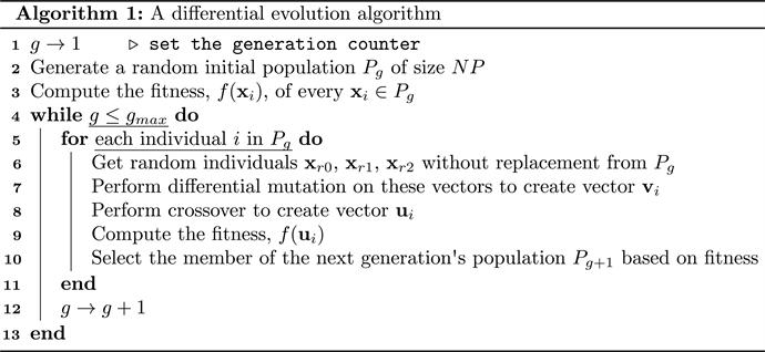
4.1. Algorithm
In this paper, we used the “DE/rand/1/bin” differential evolution strategy to find each of the BWB optimal parameters. Each parameter is encoded as a real number value, normalized to the range [0, 1]. All DE operations are performed in this range. When calculating the fitness function, these parameters are converted to their actual parameter values using (5).
These parameters define how and when to enter and exit a trade. Trades are entered only once per month, starting at the first trading day of each month. If
the entry conditions are not met, we skip to the next day, until we find a suitable day to enter the trade. This is repeated for a maximum of 10 trading days. If no suitable trade is found, we skip to the next month.
The trade parameters used, along with some sample values, (using a points based option’s strike mapping to be discussed further below), are:
1) Upper long strike, ULS, e.g. ULS = S + 1, that is, 1 point above the underlying price, S.
2) Short strike, SS, e.g. SS = S-4, that is, 4 points below the underlying price, S.
3) Lower long strike, LLS, e.g. LLS = S-12, that is, 12 points below the underlying price, S.
4) Entry days to expiration, entry DTE = 70, e.g. 70 days to expiration at entry.
5) Exit days to expiration, exit DTE = 14, e.g. 14 days to expiration to exit.
6) Maximum cost to enter a trade, e.g. 5% of required margin.
7) Minimum profit to exit a trade, e.g. 20% of maximum possible profit.
8) Maximum loss to exit a trade, e.g. 30% of required margin.
9) Points above upper long strike to prevent exit (Exit Override), e.g. 13 points.
With the sample values given above, this translates to a strategy that on the first trading day of each month, endeavors to, (by item 1) buy a long put 1 point above the underlying price, (by item 2) sell two short puts 4 points below the underlying price, and (from item 3) buy a long put 12 points below the underlying price. All put positions are from an option chain which has (by item 4) days to expiration closest to 70 days. The total BWB position cost is limited to a maximum debit of (by item 6) 5% of the required margin.
This strategy will monitor the profit/loss of each day post trade initiation, and exit the trade whenever one of the following three conditions occur: i) (by item 7) a profit target of 20% of the maximum possible profit is reached, or ii) (by item 8) a maximum loss of 30% of the required margin is reached, or iii) (by item 5) there are 14 days left until expiration. However, these three exit conditions are overridden whenever (by item 9) the current closing price is 13 points above the upper long strike. If this case holds, the strategy doesn’t exit until the options expire.
The fitness function to maximize was formulated with the consideration of obtaining a smooth equity curve, while also optimizing profits and minimizing drawdowns. Therefore the fitness function adopted to optimize the parameters is a weighted sum of three terms given by:
 (9)
(9)
where x represents the vector of trade parameters. The first term is the annualized returns divided by the annualized volatility. This ensures that the returns do not have an elevated volatility. The second term adds the final cumulative returns of the strategy to ensure to optimize the total profits made. The last term penalizes the fitness by the level of maximum equity drawdown. In addition to maximizing the fitness value the following conditions were required to be met:
· The fitness must be positive.
· The number of winning trades must be at least 70% of the total trades entered.
· The number of trades entered is at least 85% of the total trading months, where we aim to put on a trade at the beginning of each month.
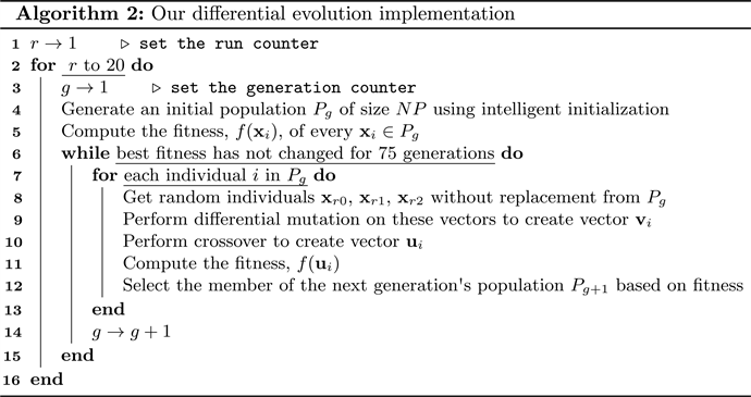
For the initial DE parent population, we used an intelligent initialization method. Since there are three conditions for the fitness to be valid, we randomly generate individuals from a uniform distribution of parameters and evaluate their fitness. Only individuals satisfying all pre-conditions were added to the initial population. This process continued until the population was complete. After forming the initial population, the DE operations of mutation and crossover were used to generate the child population to explore the fitness landscape. This was repeated until there was little variation in the best individual’s fitness. The most fit individual out of all the generations was kept. Subsequently, the whole process was repeated again for 20 runs, to fully explore the fitness landscape.
5. Implementation Details
5.1. Margin Requirement
The term margin refers to the capital required in a brokerage account in order to be able to initiate a trade. The CBOE provides a “margin manual” ( Chicago Board Options Exchange, 2000 ) for well known option strategies that outlines how to calculate the margin required for a regular trading margin account. This manual defines the margin for the traditional butterfly structure, but it does not provide guidance as to how to calculate the margin for a broken wing butterfly.
For non-conventional strategies, most brokers require a margin equal to the maximum theoretical loss the strategy can experience. Since a BWB is risk defined, the margin required can easily be calculated using this criterion.
We calculated the margin for this strategy by examining the P/L graph at expiration. The maximum loss at expiration is the margin required for the BWB. This is the level of lower expiration line of the BWB P/L plot.
5.2. Strike Mapping
Three parameters of the BWB strategy specify the strikes of the long and short puts. As the underlying price varies throughout history, a method must be used which indirectly assigns strike values. We consider three such methods and evaluate their efficacy. The three methods are:
1) Points Based Mapping
2) Delta Based Mapping
3) Normalized Strike Mapping
We will examine each of these mappings with reference to Table 1. This table shows a partial option’s chain for the SPY at EOD (end of day) for the date 04/04/2005. The expiration date for these options are 06/18/2005 which represents DTE = 75 days. The underlying (SPY) EOD closing price was $117.63. A number of different strikes are listed with the corresponding bid and ask prices as well as delta values. Note also that the last column contains the values of each strike normalized by the closing price. These are referred to as normalized values (NV). Therefore, a strike of 118 would be represented by a NV of approximately 1 (=118/117.63).
Let us consider, as an example, how the three strikes 123/120/100 can be obtained by the three mapping methods.
Points based mapping: Using this mapping the strikes are assigned by their relative point distance from the underlying EOD closing price. If we denote the EOD closing price as S then each of the strikes can be represented by S + 5.37/S + 2.37/S − 17.63. (The nearest strike is chosen when evaluations do not result in
![]()
Table 1. SPY option EOD data for date 04/04/2005. The last column represents the strike normalized values (NV).
exact strike levels). In this way the offsets from the EOD closing price for other dates in history can be used to determine the relevant strikes at other dates. This method is a widely used by option traders.
Delta based mapping: This alternative method simply specifies strikes corresponding to the absolute value of the corresponding deltas. So that strikes 123/120/100 can alternatively be specified as the 0.8/0.6/0.04 delta strikes. (Again, choose the strike nearest to the delta value.)
Normalized Strike Mapping: This last method requires that each strike in the option chain is normalized by the EOD closing price. This is shown in the last column in Table 1. In this way the strikes 123/120/100 can be referred to via their normalized values of 1.045/1.020/0.8501. (Again the closest values are sufficient). This method was introduced in ( Tymerski & Greenwood, 2018 ), where it was found to be highly effective in optimizing profits.
6. Results
6.1. BWB Parameter Optimization
The underlying considered in this paper is the S & P 500 exchange traded fund (ETF) that has the symbol SPY, which trades on NYSE Arca, which is part of the New York Securities Exchange. The option data used for optimization is the end of day (EOD) prices obtained from IVolatility.com. The data spans from January 10, 2005 to July 15, 2016.
Results were generated using a population size![]() , a mutation rate,
, a mutation rate, ![]() , and a crossover rate,
, and a crossover rate,![]() . The exploration of the fitness landscape is stopped once the best fitness has not changed for 75 generations. There were a total of 20 runs where after each run the initial population was reset. The results for all three option strike mapping methods, i.e. points, delta, and normalized strike mapping, were obtained for the single fitness function used.
. The exploration of the fitness landscape is stopped once the best fitness has not changed for 75 generations. There were a total of 20 runs where after each run the initial population was reset. The results for all three option strike mapping methods, i.e. points, delta, and normalized strike mapping, were obtained for the single fitness function used.
The ranges of values used for each parameter are shown in Table 2.
![]()
Table 2. Ranges used for each parameter for each mapping type. The symbol S, denoting the current underlying price, is used in determining the strike locations for the points mapping method. The delta values are shown in absolute terms. (In actuality, a long position will have a negative value and a short position will have positive deltas). NV represents the normalized values.
In order to ensure our algorithm produces a BWB structure, we added the following requirement:
lower long strike, LLS < short strike, SS < upper long strike, ULS.
The exit override parameter for the delta mapping method is different from the other methods. When we enter a position, we save the strike which is closest to the delta value required for future reference. For example, if we have an exit override parameter value of 0.83 delta, from Table 1 we can see that the closest strike for this delta value is $124. For the remainder of the trade, a closing value above $124 triggers the exit override condition.
The performance of the BWB using the optimized parameters for each of the mappings is shown in Table 3. Of the three mapping methods, the normalized strike mapping method achieved the highest fitness value of 2.61. As seen in the table, it also achieved the best cumulative return (of 184.3%), the second highest Sharpe ratio (of 0.85), and a modest drawdown (of 29.3%). The results of the other mapping methods are shown in Table 3 as well as simply holding SPY stock.
The optimized parameters for each mapping method are shown in Table 4. We can observe that all methods result in having the upper long strike in-the-money, the short strike slightly in-the-money, and the lower long strike
![]()
Table 3. Performance comparison from 2005 to 2016. Margin results for the BWB are per tranche (1/2/1 contracts) and per share for SPY stock.
![]()
Table 4. Optimized parameters for each of the three mapping methods. The symbol S, representing the current underlying price, is used in determining the strike locations for the points mapping method. NV represents the normalized values of the strikes.
invariably appears far out-of-the money. All mapping methods have the optimum entry days to expiration at 61 days, and the exit days to expiration at 6 - 7 days, indicating a uniformly ideal entry point and exit point. When the BWB strategy is close to expiration the build up of the profit hump is more pronounced and easier to achieve. This explains the high cumulative returns this strategy is achieving for all mapping methods. Only the normalized mapping method requires a credit when entering a trade. All the mapping methods share a small range of optimized values for exiting with a profit (of 54% to 68%) as well as a small range for optimized maximum stop losses (of 23% to 29%).
Table 5 shows the percentage of times specific exit conditions were triggered for all trades. For all mapping methods we observe that the parameter that influences the exits the most is the Exit DTE parameter. This indicates that the BWB strategy spends most of the time avoiding a maximum loss and obtaining a minimum profit. Both the points and normalized mapping methods have a similar percentage of trade exits due to maximum loss (of 14% to 17%) and of minimum profit (of 8% to 9%). They differ on the percentages of exits due to option expiration. This exit implies that the price of the underlying was above the upper long strike. A minimal loss and profit is achieved at this point. This helps explain why the normalized method has a higher volatility and higher returns.
For the delta method we observe the most variation of the exit parameters. It limits maximum loss stop outs the most, and takes the minimum profit the most as well.
Figure 3 shows the equity curves for each mapping method along with the returns of the underlying, SPY. It shows that the normalized mapping method achieves the greatest final return, but also the greatest drawdown. The points and delta methods achieve similar returns to the SPY. Compared to SPY, all methods have a lower drawdown and volatility. Figure 4 shows the beta factor each return has with their underlying, the SPY. The beta factor is a measurement of how much the returns of the strategy are explained by the underlying. In general, a beta factor close to 0 is ideal since the returns are independent of the movements in the underlying. The normalized method has the highest mean beta exposure, which explains why this strategy has a great drawdown and volatility. All mapping methods have a low beta exposure to the SPY.
Figure 5 show the returns of each strategy, clearly showing the greater volatility and returns of the normalized mapping method, and the reduced volatility of
![]()
Table 5. Percentage of total trades where each trade exit condition was met.
![]()
Figure 3. Cumulative returns comparison for all mapping methods and SPY.
![]()
Figure 4. Beta factor to SPY comparison for all mapping methods.
![]()
Figure 5. Returns comparison for all mapping methods.
the points mapping method.
Figure 6 shows the annual returns for each method. All methods have a negative return during the 2008 great financial crisis. Noticeably, all methods only
had a negative yearly return in 2008.
6.2. BWB Parameter Re-Optimization to Reduce Volatility
The volatility and drawdown for all the mapping methods shown in Table 3 can mostly be attributed to the increased gamma risk which occurs for dates near option expiration. Gamma is one of the option Greeks previously discussed. Gamma risk refers to the higher sensitivity of option prices due to underlying price variations for options nearing expiration. Our optimization resulted in finding low exit DTE parameters of just 6 and 7 days. To reduce volatility due to gamma risk, the exit DTE parameter range was changed from 1 to 30, as seen in Table 2, to a more restricted range of 12 to 30 and a re-optimization for the same fitness function was performed for all mapping methods.
Of the three mapping methods, the normalized strike mapping method again achieved the highest fitness value of 2.13, compared to 1.94 and 1.77 for the other methods. As expected, all fitness values were lower than that previously achieved under less constrained optimization. However, all mappings resulted in reduced volatility as was desired. As seen in Table 6, the normalized mapping method also achieved the best cumulative return (of 120.1%), and now highest Sharpe ratio (of 0.95), and lowest drawdown (of 14.8%). Further results comparing
![]()
Figure 6. Annual returns comparison for all mapping methods.
![]()
Table 6. Performance comparison from 2005 to 2016 with the new range of exit DTE of [12, 30]. All other ranges are as they appear in Table 2.
the performance between the mapping methods are shown in this table.
The re-optimized parameters for each mapping method are shown in Table 7. We can observe that, again, all methods result in having the upper long strike ITM, the short strike slightly ITM, and the lower long strike invariably appears FOTM. All mapping methods have the optimum entry DTE either at or close to 61 days. We observe this time the delta and normalized methods have their exit DTE at 12 - 13 days, but the points method has now increased to 24 days. All mapping methods now permit to pay a debit to enter a trade. Notice also that all methods share a small range of optimized values for exiting with a profit, of 43% to 50%, as well as a small range for ideal maximum stop loss, of 21% to 23%.
Table 8 shows what percentage of the exit conditions were triggered for all trades. For all mapping methods we observe, again, that the parameter that influences the exits the most is the Exit DTE parameter. The points mapping methods no longer has trades taken to expiration, due to it having a greater Exit DTE parameter. The normalized method takes more maximum losses and less minimum profits.
Figure 7 shows the equity curves for each mapping method along with that of the underlying, SPY. It shows the normalized mapping method achieves a similar return to the SPY, but at a lower drawdown and volatility. In Figure 8 we observe that the beta factor is reduced significantly for the normalized method.
![]()
Table 7. Re-optimized parameters for each of the three mapping method with a new range for Exit DTE parameter of [12, 30]. The symbol S used in determining the strike locations for the points mapping represents the current underlying price. NV represents the normalized value.
![]()
Table 8. Percentage of total trades where a trade exit condition was met with new ranges.
![]()
Figure 7. Cumulative returns comparison for all mapping methods and SPY.
![]()
Figure 8. Beta factor to SPY comparison for all mapping methods.
7. Trade Example
Given the optimized parameters for the normalized mapping method in Table 4, we show how a trader would enter a trade on a given day. Our parameters specify buying the upper long strike with a normalized value closest to 1.0416, selling the short strike with a normalized value closest to 1.0181, and buying the lower long strike with a normalized value closest to 0.8484. For the entry date of 4/4/2005 and referencing the option data of Table 1, we find that the closest options strikes are 123/120/100.
The strategy P/L curve is shown in Figure 9. This figure highlights the current underlying price, the expiration P/L, and the T + 0 P/L lines. The lower expiration line appears at a level of $1541 and the maximum profit is seen to be $458.
To calculate the cost of this strategy, we use a weighted sum of bid and ask values to realistically determine option prices ( Del Chicca & Larcher, 2012 ) together with the corresponding number of contracts.

![]()
Figure 9. Entry BWB on 04/04/2005. T + 0 line was modeled using the Black-Scholes-Merton formula.
Note that this value of credit received is available on an options trading platform (and so does not require any calculation by the trader in practice). For this strategy, the minimum credit we are willing to receive is 6% of $1541, which is $94. Since we received a credit of $158, we satisfy this parameter. For this strategy the stop loss is set at 29% of $1541, which is $447, and the profit taking point is at 68% of $458, which is $311. The exit override price is![]() . If the underlying price goes above this level the strategy is left to expire, in which case the profit from the trade is simply the original credit received.
. If the underlying price goes above this level the strategy is left to expire, in which case the profit from the trade is simply the original credit received.
Figure 10 shows the P/L of the strategy as it progresses towards expiration. Figure 10(a) shows a snapshot 10 days after entry. There is a slight loss on the day but nowhere near the stop loss value. Figure 10(b) shows the progress after 22 days. The strategy is still at a loss, but we are starting to see a slight buildup of the profit hump. After 39 days has passed in Figure 10(c) we notice the strategy is starting to turn around, and after 67 days, see Figure 10(d), the price has recovered and the strategy is able to exit above the minimum profit taking point of $311. Figure 11 shows the P/L evolution for the strategy, from trade initiation to exit.
8. Conclusions
In this paper, the BWB option’s strategy has been examined. In particular optimum setup and exit parameters have been chosen. The setup parameters consist of the three strike locations, DTE at trade initiation, and acceptable debit or credit limits. Exit parameters involve minimum profit, maximum loss, minimum DTE to exit as well as an exit override parameter which when satisfied permits the trade to continue to option expiration. Use of a differential evolution algorithm has been shown to be effective in achieving these aims. Two sets of optimal parameters were actually developed. One where profit was optimized and the other where a reduced level of trade volatility is achieved, albeit at the expense of profit. In the latter case, this is achieved simply by exiting the trade a few days
![]()
Figure 10. Progress of the strategy after (a) 10 days, (b) 22 days, (c) 39 days, and (d) 67 days.
![]()
Figure 11. P/L progress of the BWB strategy entered on 04/04/2005.
earlier in the trade cycle.
The issue of strike mapping, in which an indirect method is used to select strikes, was addressed. The normalized strike mapping method was found to be the most effective of the three methods considered. This method represents strikes as normalized values with respect to the current underlying price. The normalized mapping method achieves the best cumulative return out of all mapping methods. As shown in Table 4, an entry DTE of 61 days, and an exit DTE of 6 - 7 days were found to be optimal for all mapping methods. Taking profits and losses early helps with limiting the drawdown and volatility while still achieving high returns (see Table 4 and Table 5). The normalized method also has a low beta exposure to the SPY, making it ideal for achieving returns in different market conditions. As mentioned above, when limiting the exit DTE of the BWB strategy, namely exiting at a DTE of 13 days, we can limit the volatility and drawdown of the strategy (see Table 6 and the equity curves of Figure 7).
To fully examine the possibilities that the BWB strategy holds, the parameters were given a wide range of values from which to optimize. As can be seen from the trade example of the last section, this resulted in both the upper long and short strikes being ITM. Also the lower wing width was much wider than the upper wing width. Effectively the option structure became a loss limited put ratio spread. Traditionally wing spans with a 60%/40% ratio are typically used. However, over the decade of time the optimized strategy was tested the ratio spread type structure was shown to be optimal. Further work will entail limiting the initial delta of the structure to be closer to delta neutral, i.e. having a strategy delta of zero. The consequences of this will be to even out the wing spans while making the trade even less risky at trade initiation, due to its delta neutrality. However, this will be achieved with a lower profit. Future work will indicate the merits of adding this constraint on the initial strategy delta. Future work will also consider variations on the fitness function to be optimized.
In summary, the main contributions of this work can be seen as twofold: 1) an optimized structure of a Broken Wing Butterfly option strategy together with trading parameters has been provided. This was obtained through the use of a differential evolution algorithm set up to operate on a fitness function which weighed the conflicting requirements of maximizing profit, achieving equity curve linearity and minimizing the maximum drawdown, and 2) the importance of using the normalized strike mapping method has been seen to be integral in achieving the optimized performance. The results obtained have been for the SPY exchange traded fund. The procedure presented here may be applied to optimize for use with other assets, such as the SPX (S & P 500 index) and RUT (Russell 2000 index) which offer favorable tax treatment (where any gain or loss is treated for tax purposes as 40% short-term gain and 60% long-term gain), thus broadening trading possibilities.