The Expected Discounted Tax Payments on Dual Risk Model under a Dividend Threshold ()
1. Introduction
Consider the surplus process of an insurance portfolio
 (1.1)
(1.1)
which is dual to the classical Cramér-Lundberg model in risk theory that describes the surplus at time , where
  is the initial capital, the constant
  is the rate of expenses, and
  is aggregate profits process with the innovation number process
  being a renewal process whose inter-innovation times
  have common distribution
 . We also assume that the innovation sizes
 , independent of
 , forms a sequence of i.i.d. exponentially distributed random variables with exponential parameter
 . There are many possible interpretations for this model. For example, we can treat the surplus as the amount of capital of a business engaged in research and development. The company pays expenses for research, and occasional profit of random amounts arises according to a Poisson process.
Due to its practical importance, the issue of dividend strategies has received remarkable attention in the literature. De Finetti [1] considered the surplus of the company that is a discrete process and showed that the optimal strategy to maximize the expectation of the discounted dividends must be a barrier strategy. Since then, researches on dividend strategies has been carried out extensively. For some related results, the reader may consult the following publications therein: Bühlmann [2], Gerber [3], Gerber and Shiu [4,5], Lin et al. [6], Lin and pavlova [7], Dickson and Waters [8], Albrecher et al. [9], Dong et al. [10] and Ng [11]. Recently, quite a few interesting papers have been discussing risk models with tax payments of loss carry forward type. Albrecher et al. [12] investigated how the loss-carry forward tax payments affect the behavior of the dual process (1.1) with general inter-innovation times and exponential innovation sizes. More results can be seen in Albrecher and Hipp [13], Albrecher et al. [14], Ming et al. [15], Wang and Hu [16] and Liu et al. [17,18].
Now, we consider the model (1.1) under the additional assumption that tax payments are deducted according to a loss-carry forward system and dividends are paid under a threshold strategy. We rewrite the objective process as . that is, the insurance company pays tax at rate
  on the excess of each new record high of the surplus over the previous one; at the same time, dividends are paid at a constant rate
  whenever the surplus of an insurance portfolio is more than b and otherwise no dividends are paid. Then the surplus process of our model
  can be expressed as
 (1.2)
(1.2)
for , with
 . where
  is the indicator function of event
  and
and  is the surplus immediately before time
 .
.
For practical consideration, we assume that the positive safety loading condition
 (1.3)
(1.3)
holds all through this paper. The time of ruin is defined as  with
with  if
if
 for all
 .
.
For initial surplus , let
, let  be the present value of all dividends until ruin, and
  is the discount factor. Denote by
  the expectation of
 , that is,
 (1.4)
(1.4)
It needs to be mentioned that we shall drop the subscript  whenever
  is zero.
The rest of this paper is organized as follows. In Section 2, We derive the expression of  (i.e. the Laplace transform of the first upper exit time). We also discuss the expected discounted tax payments for this model and obtain its satisfied integro-differential equations. Finally, for Erlang (2) inter-innovation distribution, closed-form expressions for the the expected discounted tax payments are given.
2. Main Results and Proofs
Let  denote the Laplace transform of the upper exit time
 , which is the time until the risk process
  starting with initial capital
  up-crosses the level
  for the first time without leading to ruin before that event. In particular,
  is the probability that the process
  up-crosses the level
  before ruin.
For general innovation waiting times distribution, one can derive the integral equations for . When
 ,
,
 (2.1)
(2.1)
When ,
,
 (2.2)
(2.2)
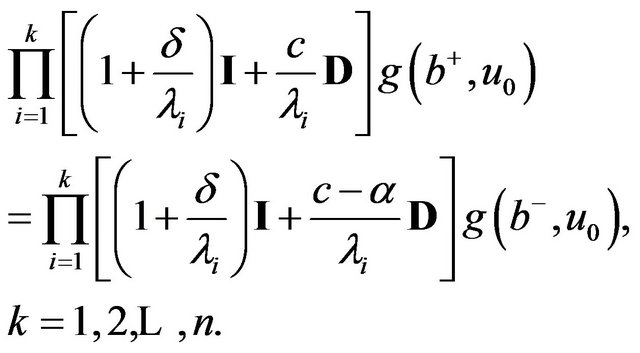
It follows from Equation (2.1) and from Equation (2.2) that  is continuous on
  as a function of
  and that
 (2.3)
(2.3)
For certain distributions , one can derive integrodifferential equations for
  and
and . Let us assume that the i.i.d innovation waiting times have a common generalized Erlang
 distribution, i.e. the
 ’s are distributed as the sum of n independent and exponentially distributed r.v.’s
  with
with  having exponential parameters
 .
.
The following theorem 2.1 gives the integro-differential equations for  when
when ’s have a generalized Erlang
 distribution.
Theorem 2.1 Let  and
and  denote the identity operator and differentiation operator respectively. Then
  satisfies the following equation for
 (2.4)
(2.4)
and
 (2.5)
(2.5)
for .
.
Proof First, we rewrite  as
as  when
when
 with
with  in the surplus process (1.2)
with . Thus, we have
 . When
 ,
,
 (2.6)
(2.6)
for , and
, and
 (2.7)
(2.7)
By changing variables in from Equation (2.6) and from Equation (2.7), we have for ,
,
 (2.8)
(2.8)
for , and
, and
 (2.9)
(2.9)
Then, differentiating both sides of from Equation (2.8) and from Equation (2.9) with respect to , one gets
 (2.10)
for , and
, and
 (2.11)
Using from Equation (2.10) and from Equation (2.11), we can derive from Equation (2.4) for  on
on .
.
Similar to from Equation (2.6) and Equation (2.7), we have for 
 (2.12)
for , and
, and
 (2.13)
Again, by changing variables in Equation (2.12) and Equation (2.13) and then differentiating them with respect to , we obtain for
 (2.14)
for , and
, and
 (2.15)
Using Equation (2.14) and Equation (2.15), we obtain Equation (2.5) for  on
on .□
.□
It needs to be mentioned that from the proof of Lemma 2.1, we know that

Therefore, Equations (2.10), (2.11), (2.14) and (2.15) yield
 (2.16)
Remark 2.1 Using a similar argument to the one used in Lemma 2.1, one can get that when the innovation waiting times follow a common generalized Erlang distribution, the expected discounted dividend payments
  satisfies the following integro-differential equation (see Liu et al. [17]).
 (2.17)
and
 (2.18)
with
 (2.19)
In addition, the boundary conditions for  are as follows:
 (2.20)
 (2.21)
with Equation (2.19).
With the preparations made above, we can now derive analytic expressions of the expected  -th moment of the accumulated discounted tax payments for the surplus process
 . We claim that the process
 shall up-cross the initial surplus level
  at least once to avoid ruin.
Now, let
 (2.22)
denote the Laplace transform of the first upper exit time , which is the time until the risk process
 starting with initial capital
  reaches a new record high for the first time without leading to ruin before that event. In particular,
  is the probability that the process
  reaches a new record high before ruin. Then the closed-form expression of the quantity
  can be calculated as follows.
When . When
 , using a simple sample path argument, we immediately have,

or, equivalently
 (2.23)
Let  and define
 (2.24)
to be the  -th taxation time point. Thus,

(2.25)
denotes the  -th moment of the accumulated discounted tax payments over the life time of the surplus process
 .
.
We will consider a recursive formula of  in the following theorem 2.2.
Theorem 2.2 When , we have
 (2.26)
and when , we have
 (2.27)
Proof Given that the after-tax excess of the surplus level over  at time
  is exponentially distributed with mean
  due to the memoryless property of the exponential distribution. By a probabilistic argument, one easily shows that for

(2.28)
Differentiating with respect to  yields

(2.29)
When , we have
 (2.30)
When , the general solution of Equation (3.20) can be expressed as

(2.31)
Due to the facts that  and
and  , we have for
 (2.32)
Now, it remains to determine the unknown constant C in Equation (3.20). The continuity of  on
on  and Equation (3.22) lead to
 (2.33)
Plugging Equation (2.33) into Equation (2.30), we arrive at Equation (2.26). □
The special case  leads to an expression for the expected discounted total sum of tax payments over the life time of the risk process
 (2.34)
for all .
.
3. Explicit Results for Erlang(2) Innovation Waiting Times
In this section, we assume that ’s are Erlang(2) distributed with parameters
  and
and . We also assume that
  (without loss of generality).
Example 3.1 Note that
 (3.1)
(3.1)
Applying the operator  to Equations (2.4) and (2.5) gives

(3.2)
and

(3.3)
The characteristic equation for Equation (3.2) is
 (3.4)
(3.4)
without loss of generality, we assume that . We know that Equation (3.4) has three real roots, say
  and
and  which satisfies

With  replace
  in Equation (3.4), we get the characteristic equation of Equation (3.3), whose roots are denoted by
  and
and  with
with

Thus, we have
 (3.5)
(3.5)
and
 (3.6)
(3.6)
where  are arbitrary constants. To determine the arbitrary constants, we insert Equations (3.5) and (3.6) into Equation (2.3) and obtain
 (3.7)
(3.7)
and
 (3.8)
(3.8)
Apply Equation (2.10) together with Equations (2.3) and (3.5) when , we get
 (3.9)
(3.9)
Insert Equation (3.5) into Equation (2.4), we have
 (3.10)
In addition, plugging Equations (3.5) and (3.6) into Equation (2.16) yields
 (3.11)
and
 (3.12)
Some calculations give
 (3.13)
with
 (3.14)
Remark 3.1 Now, we give the explicit results for
 By Equations (3.6) and (3.13), we have for
 (3.15)
with
 (3.16)
For , using the explicit expressions of
  in Liu et al. [17], we obtain
 (3.17)
with
 (3.18)
where

and

We point out that when the innovation times are exponentially distributed, one can follow the same steps to get the explicit expressions of , which coincide with the results in Albrecher et al. (2008).
Example 3.2 (The expected discounted tax payments.) Following from Equation (2.34) of Theorem 2.2 and Remark 3.1, we have for ,
,
 (3.19)
And, for , we have
 (3.20)
Then we can get that when ’s are Erlang (2) distributed with parameters
  and
and , the expresses of
  can be given by Equations (3.15) and (3.17) and the expected discounted tax payments can be given by Equation (3.20).
4. Acknowledgements
The author would like to thank Professor Ruixing Ming and Professor Guiying Fang for their useful discussions and valuable suggestions.
NOTES
#Corresponding author.