Positive Definite Solutions for the System of Nonlinear Matrix Equations X + A*Y-nA = I, Y + B*X-mB = I ()
1. Introduction
It is well known that algebraic discrete-type Riccati equations play a central role in modern control theory and signal processing. These equations arise in many important applications such as in optimal control theory, dynamic programming, stochastic filtering, statistics and other fields of pure and applied mathematics [1] -[3] .
In the last years, the nonlinear matrix equation of the form
 (1.1)
(1.1)
where  and
and  maps from positive definite matrices into positive definite matrices is studied in many papers [4] -[8] . It is well known that Equation (1.1) with
  and
and  is a special case of algebraic discrete-type Riccati equation of the form [2] [3]
 (1.2)
(1.2)
In addition, the system (Sys.) of algebraic discrete-type Riccati equations appears in many applications [9] -[12] . Czornik and Swierniak [10] have studied the lower bounds for eigenvalues and matrix lower bound of a solution for the special case of the System:
 (1.3)
(1.3)
where .
.
In the same manner, we can deduce a system of nonlinear matrix equations as matrix Equation (1.1) with  and
and . For that, Al-Dubiban [13] have studied the system
 (1.4)
(1.4)
which is a special case of Sys.(1.3). The author obtained sufficient conditions for existence of a positive definite solution of Sys.(1.4) and considered an iterative method to calculate the solution. Recently, similar kinds of Sys.(1.4) have been studied in some papers [14] [15] .
In this paper we consider the system of nonlinear matrix equations that can be expressed in the form:
 (1.5)
(1.5)
where  are two positive integers, X, Y are
  unknown matrices, I is the
  identity matrix, and A, B are nonsingular matrices. All matrices are defined over the complex field. The paper is organized as follows: in Section 2, we derive the necessary and sufficient conditions for the existence the solution to the Sys.(1.5). In Section 3, we introduce an iterative method to obtain the positive definite solutions of Sys.(1.5). We discuss the convergence of this iterative method. Section 4 discussed the error and the residual error. Some numerical examples are given to illustrate the efficiency for suggested method in Section 5.
The following notations are used throughout the rest of the paper. The notation 
 means that
  is positive semidefinite (positive definite),
  denotes the complex conjugate transpose of
 , and
, and  is the identity matrix. Moreover,
 is used as a different notation for
 . We denote by
  the spectral radius of
 ;
;  means the eigenvalues of
  and
and  respectively. The norm used in this paper is the spectral norm of the matrix
 , i.e.
  unless otherwise noted.
2. Existence Conditions of the Solutions
In this section, we will discuss some properties of the solutions for Sys.(1.5) and obtain the necessary and sufficient conditions for the existence of the solutions of the Sys.(1.5).
Theorem 1 If  are the smallest and the largest eigenvalues of a solution
  of Sys.(1.5), respectively, and
  are the smallest and the largest eigenvalues of a solution
  of Sys.(1.5), respectively,
  are eigenvalues of A, B then
 (1.6)
(1.6)
 (1.7)
(1.7)
Proof: Let  be an eigenvector corresponding to an eigenvalue
  of the matrix A and
 ,
,  be an eigenvector corresponding to an eigenvalue
  of the matrix B and
 . Since the solution
  of Sys.(1.5) is a positive definite solution then
  and
and .
.
From the Sys.(1.5), we have


i.e

Hence

Also, from the Sys.(1.5), we have


i.e

Hence

Theorem 2 If Sys.(1.5) has a positive definite solution , then
 (1.8)
(1.8)
 (1.9)
(1.9)
Proof: Since  be a positive definite solution of Sys.(1.5), then

From the inequality , we have
 , therefore

From the inequality , we have
 , then

And from the inequality  , we have
 , therefore

From the inequality , we have
 , hence

which complete the proof.
Corollary 1 If Sys.(1.5) has a positive definite solution , then
 (1.10)
 (1.11)
Theorem 3 Sys. (1.5) has a positive definite solution  if and only if the matrices A, B have the factorization
 (1.12)
where  are nonsingular matrices satisfying the following system
 (1.13)
In this case the solution is .
.
Proof: Let Sys.(1.5) has a positive definite solution , then
 , where
  are nonsingular matrices. Furthermore Sys.(1.5) can be rewritten as


Let ,
,  , then
 ,
,  , and Sys. (1.5) turns into Sys.
(1.13).
Conversely, if  have the factorization (1.12) and satisfying Sys.(1.13), let
 , then
  are positive definite matrices , and we have


Hence Sys.(1.5) has a positive definite solution.
3. Iterative Method for the System
In this section, we will investigate the iterative solution of the Sys.(1.5). From this section to the end of the paper we will consider the matrices A, B are normal satisfing  and
and .
.
Let us consider the iterative processes
 (1.14)
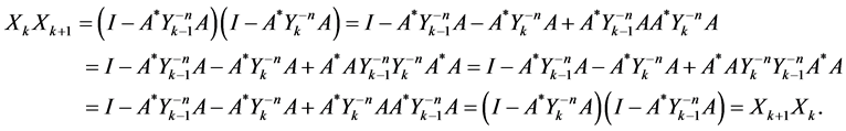
Lemma 1 For the Sys.(1.5), we have
 (1.15)
where  are matrices generated from the sequences (1.14).
Proof: Since , then

Using the conditions , we obtain

Also, we have

Using the conditions , we obtain

By the same manner, we get

Further, assume that for each , we have
 (1.16)
Now, by induction, we will prove

Since the two matrices A, B are normal, then by using the equalities (0.16), we have

Similarly

By using the conditions  and the equalities (1.16), we have

Also,we can prove

Therefore, the equalities (1.15) are true for all .
.
Lemma 2 For the Sys.(1.5), we have
 (1.17)
where  are matrices generated from the sequences (1.14).
Proof: Since  then
then 
By using the equalities (1.15), we have

Similarly we get

Further, assume that for each  it is satisfied
 (1.18)
Now, by induction, we will prove

From the equalities (1.18), we have
 (1.19)
By using the equalities (1.15) and (1.19), we have
By the same manner, we can prove

Therefore, the equalities (1.17) are true for all .
.
Theorem 4 If A, B are satisfying the following conditions:
(i) 
(ii) 
where , then the Sys.(1.5) has a positive definite solution.
Proof: We consider the sequences (1.14). For  we have
 .
.
For  we obtain

Applying the condition  we obtain

i.e.

Also, we can prove that

So, assume that
 (1.20)
Now, we will prove  and
and 
By using the in equalities (1.20) we have

Similarly

Also, by using the conditions  and the equalities (1.20), we have

Similarly, we have

Therefore, the inequalities (1.20) are true for all . Hence
  is monotonically decreasing and bounded from below by the matrix
 . Consequently the sequence
  converges to a positive definite solution X. Also, the sequence
  is monotonically decreasing and bounded from below by the matrix
and converges to a positive definite solution . So
. So  is a positive definite solution of Sys.(1.5).
4. Estimation of the Errors
Theorem 5 If A, B are satisfying the following conditions
(i) 
(ii) 
then
 (1.21)
 (1.22)
where ,
,  are matrices generated from the sequences (1.14).
Proof: From Theorem 4 it follows that the sequences (1.14) are convergent to a positive definite solution of Sys.(1.5). We consider the spectral norm of the matrices .
.

According to Theorem 4 we have

Consequently

Then we get
 (1.23)
Also, we have
According to Theorem 4 we have

Consequently

then we get
 (1.24)
By using (1.24) in (1.23), we have

Similarly, by using (1.23) in (1.24), we have

Theorem 6 If A, B are satisfying the following conditions:
(i) 
(ii) 
where , and after s iterative steps of the iterative process (1.14), we have
  , then
 (1.25)
 (1.26)
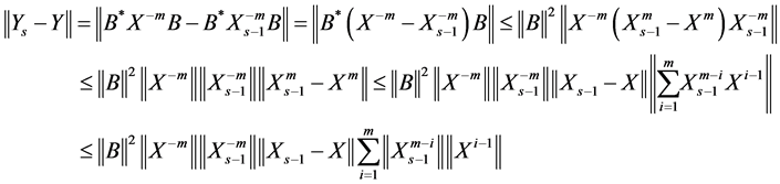
Proof: Since

Taking the norm of both sides, we have

Also,

Taking the norm of both sides, we get

5. Numerical Examples
In this section the numerical examples are given to display the flexibility of the method. The solutions are computed for some different matrices A, B with different orders. In the following examples we denote X, Y the solutions which are obtained by iterative method (1.14) and
 .
.
Example 1 Consider Sys.(1.5) with  and normal matrices

and

By computation, we get


The results are given in the Table1
Example 2 Consider Sys.(1.5) with  and matrices

and

By computation, we get


Table 1. Error analysis for Example 1.
Table 2. Error analysis for Example 2.


The results are given in Table2