1. Introduction
The classical Cayley-Hamilton theorem [1-4] says that every square matrix satisfies its own characteristic equation. The Cayley-Hamilton theorem has been extended to rectangular matrices [5,6], block matrices [7,8], pairs of commuting matrices [9-11] and standard and singular two-dimensional linear systems [5,12]. The CayleyHamilton theorem has been extended to n-dimensional systems [13]. An extension of the Cayley-Hamilton theorem for 2D continuous discrete-time linear systems has been given in [14].
The Cayley-Hamilton theorem and its generalizations have been used in control systems [14,15] and also automation and control in [16,17], electronics and circuit theory [6], time-systems with delays [18-20], singular 2-D linear systems [5], 2-D continuous discrete linear systems [12], automation and electrotechnics [21], etc.
In this paper an overview of generalization of the Cayley-Hamilton theorem is presented. The linear polynomial matrix  of det
  in the classical Cayley-Hamilton theorem is replaced by the general polynomial matrix

where  for
for  are square matrices of the same order. In the Theorem 1 given below it is proved that if
  and whenever for a square matrix A
  implies
 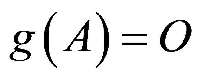 also. The converse of Theorem 1 is not true, is illustrated with the help of examples 1 and 2 in which the leading coefficient matrix of the polynomial matrix
  may be singular or non-singular. A relation between the coefficients of the polynomial
  and the coefficient matrices of
  is worked out in corollaries 1, 2 and 3.
2. Preliminaries
Lemma 1. If the elements of a matrix A are polynomials in x of degree ≤ n, then A can be expressed as a polynomial matrix  in x of degree ≤ n, where the matrices
  are of the same order as that of the matrix A.
Illustration 1. Let

be a matrix of order 3 × 3. Then
 where
where
 ;
; ;
;
 and
and 
Lemma 2. If A is a square matrix of order n having elements as polynomials in x each of degree ≤ m, then the elements of the adjoint of the matrix A are also polynomials in x of degree .
.
Illustration 2. Let

be a matrix of order 3 × 3 having elements as polynomials in x of degree ≤ 4, then
 where
where  denotes the
  th element of the adjA, a polynomial in x of degree ≤ r. For instance in adjA, the element at the (2.1) th position is
 .
.
Hence by the Lemma 1, because adjA contains elements as polynomials in x of degree ≤ 8, it implies that  , where each of the
 ,
,  is also a square matrix of order 3.
Remark 1. Prior to understand the concept in the proof of the main Theorem 1 given below, we first consider the following two illustrations of polynomial matrix  having the leading coefficient matrix singular or non-singular such that if
  and for a square matrix A, whenever

Illustration 3: Let
 (2.1)
(2.1)
be a polynomial matrix over  for
for
 where A2 is a non-singular matrix and
  denotes the set of all 2 × 2 matrices whose elements are polynomials in x over the field F. Then there exists a matrix
 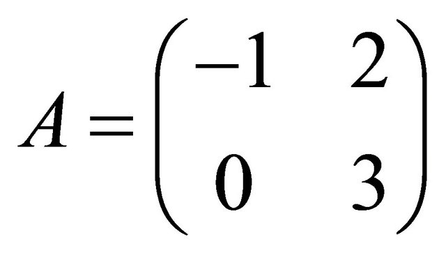 such that;
Also from (2.1), we have

Hence,  implies
Illustration 4: Consider the polynomial matrix
 (2.2)
(2.2)
over , for
, for ;
;  and
and , where the leading coefficient matrix A2 is singular. Then there exists a matrix
  such that

From (2.2), we have
As in Illustration 3, it can be easily verified that

3. Main Results
Theorem 1. Let  be a polynomial matrix for
  where
where  for
for , are square matrices of order n over the field F. If
 , then whenever
  (Zero matrix) implies
  Converse is not true.
Proof. Since
 (3.1)
(3.1)
is itself is a matrix of order n × n having elements as polynomials in x each of degree ≤ m, therefore, using lemma 2, we have
 (3.2)
(3.2)
Also  is a polynomial in x over
  of degree ≤ mn. Therefore, using Lemma 1, we have
 (3.3)
(3.3)
Since for any square matrix A, we have;
 (3.4)
(3.4)
where I is the identity matrix of the same order as of A. Now using (3.4), we have
 (3.5)
(3.5)
Therefore, using (3.1) to (3.3) above, we have from (3.5)
 (3.6)
(3.6)
Comparing coefficients of the corresponding terms on both sides of Equation (3.6), we get
 . (3.7)
Multiplying the equations in (3.7) by the matrices

respectively and adding, we obtain;

Converse is not true. For this consider the following examples with the coefficient matrix singular and nonsingular respectively.
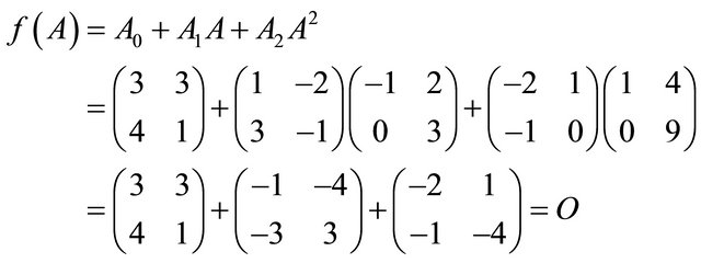
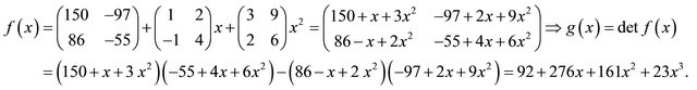
Example 1. Consider the function ; where

Then for the scalar matrix , we have
 Whereas,

Example 2: Consider the function  ; where

Then there exist infinite number of matrices A over the complex numbers C of the form

or

for , such that
  but
but .
.
For instance, if ,
,  , then

Whereas,

Illustration 5. For  in Theorem 1, let

be a polynomial matrix in ,where
  such that
  for some square matrix A of order 3.
 . (3.8)
Since the elements of the matrix  are polynomials in x of degree

is a polynomial in x over the field F of degree ≤ 9. Therefore, let
 (3.9)
(3.9)
Also each element of the  being a polynomial in x of deg ≤ 6. So by Lemma (2), let
 (3.10)
Now using (3.4), we have
 (3.11)
Comparing the coefficients of the equivalent powers of x on both sides, we have
 (3.12)
Multiplying these equations by  respectively and adding, we get;

Corollary 1. If  and
and  be the polynomials given in (3.1) and (3.3) respectively, then for
 .
.
Therefore, the constant term  of the polynomial
  is the determinant of the constant term
  in the polynomial matrix
 .
.
Corollary 2. From (3.1) and (3.3), for  , we have
 (3.13)
Therefore, in case for , when
  or
or , then from (3.13), we have
 (3.14)
Therefore, if , then from (3.14), we get
  . Hence if,
 .
.
Thus  if the leading coefficient matrix
  in
in  is singular.
Corollary 3. If

be a bi-quadratic polynomial matrix for
and if

Then we have,

and so on.
In general, for any ; we have pn = coefficient of
 , for
, for ;
; ,
, .
.
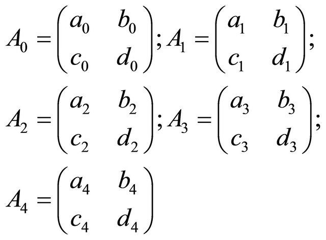
Example 3. Consider the cubic polynomial matrix
 where for
 ,
,  , if we have

where , the coefficient of
  is given by
 (3.15)
It can be easily verified that

and

Similarly coefficients of the other powers of x, i.e.,  can be found by using (3.15). For instance

which verifies our assertion.
4. Conclusion
The concept of the Theorem 1 given above and the relation in (3.15) can be generalized to any polynomial matrix of arbitrary degree with coefficients as square matrices of any order.
5. Acknowledgements
The author wishes to thank Dr. P. L. Sharma, Associate Professor Department of Mathematics and Statistics of the H. P. University Shimla (H.P.) India for his help and guidance. He also expresses his gratitude to the Govt. of Himachal Pradesh Department of Higher Education for granting him study leave to complete the assigned project.