On the Stability and Boundedness of Solutions of Certain Non-Autonomous Delay Differential Equation of Third Order ()
Received 23 January 2016; accepted 21 March 2016; published 24 March 2016

1. Introduction
This paper considers the third order non-autonomous nonlinear delay differential
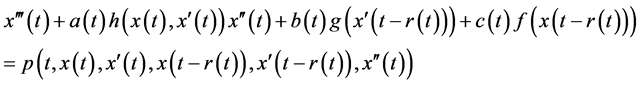 (1.1)
(1.1)
or its equivalent system
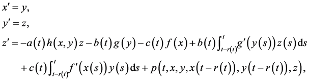 (1.2)
(1.2)
where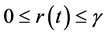 ,
,  ,
,  , β and
  are some positive constants,
  will be determined later,
  ,
,  ,
,  are real valued functions continuous in their respective arguments on
 ,
,  ,
,  ,
,  ,
,  ,
, ![]() and
and ![]() respectively and
respectively and![]() . Besides, it is supposed that the derivatives
. Besides, it is supposed that the derivatives![]() ,
, ![]() are continuous for all x, y, with
are continuous for all x, y, with![]() . In addition, it is also assumed that the functions
. In addition, it is also assumed that the functions![]() ,
, ![]() ,
,![]() and
and ![]() satisfy a Lipschitz condition in
satisfy a Lipschitz condition in ![]()
![]() and z; throughout the paper
and z; throughout the paper![]() ,
, ![]() and
and ![]() are respectively abbreviated as x, y and z. Then the solutions of (1.1) are unique.
are respectively abbreviated as x, y and z. Then the solutions of (1.1) are unique.
In applied science, some practical problems are associated with Equation (1.1) such as after effect, nonlinear oscillations, biological systems and equations with deviating arguments (see [1] - [3] ). It is well known that the stability of solutions plays a key role in characterizing the behavior of nonlinear delay differential equations. Stability is much more complicated for delay equations. Thus, it is worthwhile to continue to investigate the stability and boundedness of solutions of Equation (1.1) and its various forms.
Equation of the form (1.1) in which![]() ,
, ![]() and
and ![]() are constants has been studied by several authors Sadek [4] [5] , Zhu [6] , Afuwape and Omeike [7] , Ademola and Aramowo [8] , Yao and Meng [9] , Tunc [3] and Ademola et al [10] to mention a few. They obtain the stability, uniform boundedness and uniform ultimate boundedness of solutions. In a sequence of results, Omeike [11] considers the following nonlinear delay differential equation of the third order, with a constant deviating argument r,
are constants has been studied by several authors Sadek [4] [5] , Zhu [6] , Afuwape and Omeike [7] , Ademola and Aramowo [8] , Yao and Meng [9] , Tunc [3] and Ademola et al [10] to mention a few. They obtain the stability, uniform boundedness and uniform ultimate boundedness of solutions. In a sequence of results, Omeike [11] considers the following nonlinear delay differential equation of the third order, with a constant deviating argument r,
![]()
and established conditions for the stability and boundedness of solution when ![]() and
and ![]() while Tunc [12] considers a similar system with a constant deviating argument r of the form
while Tunc [12] considers a similar system with a constant deviating argument r of the form
![]()
and obtains the conditions for its boundedness of solution.
Results obtained are now extended to non-autonomous delay differential Equation (1.1). Results obtained in this work are comparable in generality to the results of Sadek [7] on analogous third order differential equation which itself generalizes an analogous third-order results of Zhu [5] , and also complement existing results on third order delay differential equations. We establish sufficient conditions for the stability (when![]() ) and boundedness (when
) and boundedness (when![]() ) of solutions of Equation (1.1) which extend and improve the results of Omeike [11] and Tunc [12] . An example is given to illustrate the correctness and significance of the result obtained.
) of solutions of Equation (1.1) which extend and improve the results of Omeike [11] and Tunc [12] . An example is given to illustrate the correctness and significance of the result obtained.
Now, we will state the stability criteria for the general non-autonomous delay differential system. We consider:
![]() (1.3)
(1.3)
where ![]() is a continuous mapping,
is a continuous mapping,
![]()
and for![]() , there exists
, there exists![]() , with
, with
![]()
Definition 1.0.1 ( [8] ) An element ![]() is in the
is in the ![]() -limit set of
-limit set of![]() , say,
, say, ![]() , if
, if ![]() is defined on
is defined on ![]() and there is a sequence
and there is a sequence![]() ,
, ![]() as
as![]() , with
, with ![]() as
as ![]() where
where
![]()
Definition 1.0.2 ( [8] [13] ) A set ![]() is an invariant set if for any
is an invariant set if for any![]() , the solution of (1.2),
, the solution of (1.2), ![]() , is defined on
, is defined on ![]() and
and ![]() for
for![]() .
.
Lemma 1 ([8,13]) An element ![]() is such that the solution
is such that the solution ![]() of (1.3) with
of (1.3) with ![]() is defined on
is defined on ![]() and
and ![]() for
for![]() , then
, then ![]() is a non-empty, compact, invariant set and
is a non-empty, compact, invariant set and
![]()
Lemma 2 ( [8] [13] ) Let ![]() be a continuous functional satisfying a local Lipschitz con- dition.
be a continuous functional satisfying a local Lipschitz con- dition.![]() , and such that:
, and such that:
1) ![]() where
where![]() ,
, ![]() are wedges;
are wedges;
2) ![]() for
for ![]()
Then the zero solution of (1.3) is uniformly stable. If we define![]() , then the zero solution of (1.3) is asymptotically stable provided that the largest invariant set in Z is
, then the zero solution of (1.3) is asymptotically stable provided that the largest invariant set in Z is![]() .
.
The following will be our main stability result (when![]() ) for (1.1).
) for (1.1).
2. Statement of Results
Theorem 1 In addition to the basic assumptions imposed on the functions a(t), b(t), c(t), ![]() and p, let us assume that there exist positive constants
and p, let us assume that there exist positive constants ![]() such that the following conditions are satisfied:
such that the following conditions are satisfied:
1)![]() ;
;![]() ,
, ![]() ,
,![]() ;
;
2)![]() ;
;![]() ,
,![]() ;
;
3)![]() ;
; ![]() and
and![]() ;
;
4)![]() ;
; ![]() and
and![]() ,
, ![]() , for all x, y.
, for all x, y.
Then, the zero solution of system (1.2) is asymptotically stable, provided that
![]() (2.1)
(2.1)
and
![]() (2.2)
(2.2)
Proof
Our main tool is the following Lyapunov functional ![]() defined as
defined as
![]() (2.3)
(2.3)
where ![]() and
and ![]() are positive constants which will be determined later.
are positive constants which will be determined later.
We also assume that
![]()
where![]() .
.
By the assumption ![]() and
and![]() , from (2.3) we have
, from (2.3) we have
![]() (2.4)
(2.4)
The Lyapunov functional (2.4) can be arranged in the form
![]() (2.5)
(2.5)
From Theorem 1, ![]() and
and ![]() which makes
which makes![]() .
.
Thus, there is a ![]() such that
such that
![]() (2.6)
(2.6)
By (2) and (3) of Theorem 1, we have that the third term on the right in (2.5)
![]() (2.7)
(2.7)
and next two terms give
![]() (2.8)
(2.8)
Using (2.6), (2.7) and (2.8) in (2.5), we have
![]() (2.9)
(2.9)
where
![]()
and integrals
![]()
Thus, for some positive constants ![]() and
and![]() , where
, where ![]() small enough such that
small enough such that
![]() (2.10)
(2.10)
For the time derivative of the Lyapunov functional (2.3), along a trajectory of the system (1.2), we have
![]()
From (4) of Theorem 1, ![]() ,
, ![]() and using
and using![]() , we have that
, we have that
![]() (2.11)
(2.11)
Similarly, we obtain
![]() (2.12)
(2.12)
Thus,
![]()
If![]() , then
, then![]() . If
. If![]() , we can rewrite the term as
, we can rewrite the term as
![]() (2.13)
(2.13)
where by (3) of Theorem 1,![]() .
.
And by (1) and (2) of Theorem 1,
![]()
as
![]() (2.14)
(2.14)
According to (2) of Theorem 1, ![]() and by (3),
and by (3), ![]() and certainly
and certainly ![]() thus,
thus,
![]() (2.15)
(2.15)
![]()
and by (3) and (4) of Theorem 1, we have that
![]()
for all ![]() and
and![]() .
.
Thus, from (2.11), (2.12), (2.13), (2.14) and (2.15), we have
![]()
If we choose
![]()
and
![]()
and using![]() , we obtain
, we obtain
![]()
Choosing
![]()
we have
![]() (2.16)
(2.16)
for some![]() .
.
Finally, it follows that ![]() if and only if
if and only if![]() ,
, ![]() for
for ![]() and for
and for![]() .
.
Thus, (2.10) and (2.16) and the last statement agreed with Lemma 2. This shows that the trivial solution of (1.1) is asymptotically stable.
Hence, the proof of the Theorem 1 is now complete.
Remark 2.1 If ![]() is a constant and (1.1) is the constant co-efficient delay differential equation
is a constant and (1.1) is the constant co-efficient delay differential equation ![]() , then conditions (1)-(4) reduce to the Routh-Hurwitz conditions a > 0, c > 0 and
, then conditions (1)-(4) reduce to the Routh-Hurwitz conditions a > 0, c > 0 and![]() . To show this we set
. To show this we set ![]() and
and![]() ,
, ![]() and
and![]() .
.
Remark 2.2 If ![]() and
and ![]() in (1.1), the non-autonomous Equation (1.1) reduces to the autonomous equation considered in Sadek [4] .
in (1.1), the non-autonomous Equation (1.1) reduces to the autonomous equation considered in Sadek [4] .
3. The Boundedness of Solution
Theorem 2 We assume that all the assumptions of Theorem 1 and
![]()
![]()
hold, where ![]() is a positive constant.
is a positive constant.
Then, there exists a finite positive constant K such that the solution ![]() of Equation (1.1) defined by the initial function
of Equation (1.1) defined by the initial function
![]()
satisfies the inequalities
![]()
for all![]() , where
, where ![]() provided that
provided that
![]()
Proof of Theorem 2
As in Theorem 1, the proof of Theorem 2 depends on the scalar differentiable Lyapunov function ![]() defined in (2.3).
defined in (2.3).
Since![]() , in (1.1).
, in (1.1).
In view of (2.16),
![]()
Since ![]() for all
for all ![]() thus
thus
![]()
Hence, it follows that
![]()
for a constant![]() , where
, where![]() .
.
Making use of the inequalities ![]() and
and![]() , it is clear that
, it is clear that
![]()
By (2.10), we have![]() ,
,
Hence,
![]()
or
![]()
where![]() .
.
Multiplying each side of this inequality by the integrating factor![]() , we get
, we get
![]()
Integrating each side of this inequality from 0 to t, we get, where![]() ,
,
![]()
or
![]()
Since ![]() and using the fact that
and using the fact that ![]() for all t, this implies
for all t, this implies
![]()
Now, since the right-hand side is a constant, and since ![]() as
as![]() , it follows that there exist a
, it follows that there exist a ![]() such that
such that
![]()
From the Equation (1.1) this implies
![]()
The proof of Theorem 2 is now complete.
Remark 3.1 If ![]() is a constant,
is a constant, ![]() ,
, ![]() and
and ![]() in (1.1), the result obtained reduces to Omeike [6] and a result of Tunc [10] .
in (1.1), the result obtained reduces to Omeike [6] and a result of Tunc [10] .
4. Conclusions
The solutions of the third-order non-autonomous delay system are asymptotically stable and bounded according to the Lyapunov’s theory if the inequalities (2.1) and (2.2) are satisfied.
Example 3.1 We consider non-autonomous third-order delay differential equation
![]() (3.1)
(3.1)
with equivalent system of (3.1) as:
![]() (3.2)
(3.2)
comparing (1.2) with (3.2), it is easy to see that
![]()
![]()
![]()
The function![]() , it is clear from the equation that
, it is clear from the equation that
![]()
The function![]() , it is clear from the equation that
, it is clear from the equation that
![]()
![]()
![]()
![]()
![]()
![]()
also,
![]()
![]()
![]()
Since
![]()
we have
![]()
It follows that![]() , if the delay is increased beyond this range a limit cycle appear, followed even-
, if the delay is increased beyond this range a limit cycle appear, followed even-
tually by a period-doubling cascade leading to chaos.
Finally,
![]()
and
![]()
Thus, all assumptions of Theorem 1 and Theorem 2 are held. That is, zero solution of Equation (1.1) is asymptotically stable and all the solutions of the same equation are bounded.
NOTES
![]()
*Corresponding author.