Global Analysis of Beddington-DeAngelis Type Chemostat Model with Nutrient Recycling and Impulsive Input ()
1. Introduction
The chemostat is an important and basic laboratory apparatus for culturing microorganisms. It can be used to investigate microbial growth and has the advantage that parameters are easily measurable. The chemostat plays an important role in bioprocessing, hence the model has been studied by more and more people. Chemostats with periodic inputs were studied [1,2], those with periodic washout rate [3,4], and those with periodic input and washout [5]. In recent years, those with nutrient recycling [6-10] have been investigated and some investing results were obtained. Now many scholars pointed out that it was necessary to consider models with periodic perturbations, since those phenomena might be exposed in many real words. However, there are some other perturbations such as floods, fires and drainaye of sewage which are not suitable to be considered continually. Those perturbations bring sudden changes to the system. Systems with sudden changes are involving in impulsive differential equations which have been studied intensively and systematically [11-13]. Impulsive differential equations are found in almost every domain of applied sciences.
Recently, many papers studied chemostat model with impulsive effect the Lotka-Volterra type or Monod type functional response. But there are few papers which study a chemostat model with Beddington-DeAngelis functional response, especially a Beddinton-DeAngelis type chemostat with nutrient recycling. The BeddingtonDeAngelis functional response is introduced by Beddington and DeAngelis [14,15]. It is similar to the wellknown Holling II functional response but has an extra term  in the denominator that models mutual interference in species. The model, we consider in this paper, takes the form:
 (1)
(1)
where S(t),  represent the concentration of limiting substrate and the microorganism respectively, D is the dilution rate, a is the uptake constant of the microorganism, k is the yield of the microorganism
  per unit mass of substrate, r is the death rate of microorganism, b is the fraction of the nutrient recycled by bacterial decomposition of the dead microorganism, p is the amount of limiting substrate pulsed each T, T is the period of pulsing. Obviously, we have
  and
and . D, A, B, k, a, p are all positive constants.
The organization of this paper is as the following. In Section 2, we introduce some useful notations and lemmas. In Section 3, we will state and prove the main results on the global asymptotic stability and permanence. In Section 4, we give a brief discussion and the numerical analysis.
2. Preliminaries
In this section, we will give some notations and lemmas which will be used for our main results. Firstly, for convenience, we set  , then system (1) becomes
 (2)
(2)
Let .
.  ,
,  ,
,  is left continuous at t = nT and x(t) is continuous at t = nT.
Lemma 1. Suppose  is any solution of system (2) with initial solution
 . Then
  for all
 . Moreover, if
  then
then  for all
 .
.
The proof of Lemma 1 is simple, we omit it here.
In what follows, we give some basic properties about the following system.
 (3)
(3)
Clearly,

is a positive periodic solution of system (3). Any solution of system (3) is

Hence, we have the following result.
Lemma 2. System (3) has a positive periodic solution  and
and , as
, as  for any solution u(t) of system (3). Moreover,
  if
if  and
and  and
and  .
.
The proof of Lemma 2 can be found in [16].
Lemma 3. There exists a constant M > 0 such that S(t) < M, x(t) < M for each solution of (S(t); x(t)) system (2), for t large enough.
Proof Let (S(t); x(t)) be any solution of system (2) with initial value . Define a function
 .
.
Then

From the comparison theorem of impulsive differential equations, we have  for all t¸ 0, where u(t) is the solution of system (3). From Lemma 2, we have
  as
as , where

Hence,

Thus, V(t) is ultimately bounded. From the definition of V(t), there exists a constant
such that S(t) < M, x(t) < M for any solution (S(t), x(t)) of system (2), for t large enough. This completes the proof.
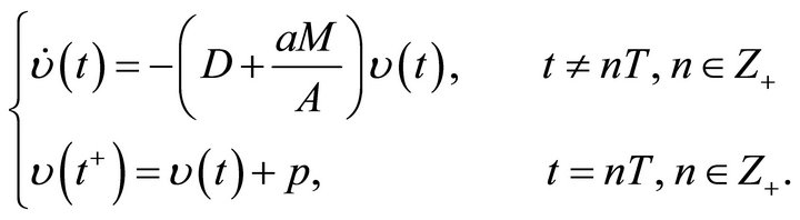
The solution of system (2) corresponding to x(t) = 0 is called microorganism-free periodic solution. For system (2), if we choose , then system (2) becomes to the following system
 (4)
(4)
System (4) has a unique global uniformly attractive positive solution

Hence, system (2) has a positive periodic solution  at which microorganism culture fails. In the next section, we will study the global asymptotical stability of the microorganism-free periodic solution
  as a solution of system (2).
3. Main Results
Theorem 1. Suppose
 (5)
(5)
Then periodic solution  of system (2) is globally attractive.
Proof Let ( ,
, ) be any positive solution of system (2). Define a function as follows

Then similar to the proof of Lemma 3, we obtain  for all
  where u(t) is the solution of system (3) and
  as
as . Hence, there exists a function
  satisfying
  as
as  such that

By the definition of , we have

It follows from the second equation of system (2) that
 (6)
(6)
From condition (5), for any enough small  we have

Since  which gives

Hence, there exist constants  and
and , such that
 (7)
(7)
If  for all
 , then from (6) we have
 (8)
(8)
For any , we choose an integer
  such that
  then integrating (8) from
  to t, from (7) we have
 (9)
(9)
where  and M is given in Lemma 3. Since
  as
as , from (9) we have
  as
as , which is a contradiction. Hencethere is a
 , T0, such that
 .
.
Now, we claim that there exists a constant  such that
In fact, if there exists a  such that
 , then there exists a
  such that
  and
and  for
for . Choose an integer
  such that
  Since for any

 (10)
(10)
integrating the above inequality from t2 to t1, from (7) we obtain (10).
Obviously, let , then from (10) we obtain a contradiction. Hence,
  for all
 . Since
  is arbitrary, we finally have
 .
.
This completes the proof.
Theorem 2. Suppose
 (11)
(11)
Then system (2) is permanent.
Proof Let (S(t); x(t)) be any solution of system (2) with initial value . By Lemma 3, the first equation of system (2) becomes

Using Lemma 2 and the comparison theorem of impulsive differential equation, we obtain  for all,
  where
where  is the solution of the following impulsive system
with initial condition . Further from Lemma 2, we have

where

Therefore, we finally obtain

This shows that S(t) in system (2) is permanent.
In the following, we want to find a constant , such that
  for t large enough.
Since

we can chose a constant  small enough such that

Consider the following auxiliary impulsive system
 (12)
(12)
from Lemma 2, system (12) has a globally uniformly attractive positive periodic solution

Since , for above
 , there is a
  and
and  such that
 (13)
(13)
Further, for above  and M > 0, where M is given in Lemma 3, there is a
  such that for any
  and
and  we have
 (14)
(14)
where  is the solution of system (12) with initial condition
 .
.
For any  ¸ if
¸ if  for all
 , then from system (2) we have

By the comparison theorem of impulsive differential equations, we have  for
for , where y(t) is the solution of system (12) with initial condition
 . From (14) we have

Hence, from (13) we further have

From the second equation of system (2) we have
 (15)
(15)
Let  such that
 . Integrating (15) on
  for all
 , we have

Hence,  for all
 . Then we have
 , which is a contradiction. Hence, there exists a
  such that
 .
.
If  for all
 , then our goal is obtained. Hence, we need only to consider these solutions which are oscillatory about
 . Let
. Let  and
and  be two large enough times such that
  and
and  for all
 . When
 , since

integrating this inequality for any , we have
 (16)
(16)
Let . For any
 , if
, if , then according to the above discussing on the case of
 , we also have inequality (16). Particularly, we obtain
 , since
  for all
 , from system (2) we have

Hence, from the comparison theorem of impulsive differential equations, we have  for all
 , where y(t) is the solution of system (12) with initial condition
 . From (14), we have

Further from (13), we also have

Thus, from system (2), we have
 (17)
(17)
For any , we choose an integer
  such that
 .
.
Integrating (17) from  to t, we have

where
From the above discussion, we have , and
, and  is independent of any solution (S(t); x(t)) of system (2). This completes the proof.
As a consequence of Theorem 1 and Theorem 2, we have the following corollary.
Corollary 1 For system (2), the following conclusions hold.
a) The microorganism-extinction solution  is globally attractive if and only if

b) The microorganism x(t) of System (2) is permanent if and only if

4. Discussion and Numerical Analysis
In this paper, we investigate Beddington-DeAngelis type chemostat with nutrient recycling and impulsive input. We prove that the microorganism-free periodic solution of the system (2) is globally attractive. The necessary and sufficient condition for permanence of system (2) are obtained in this paper.
According to Theorem 1, the microorganism-free periodic solution  is globally attractive if (5) hold. That is, this kind of microorganisms can not be cultivated under this condition. Suppose that
  and set

Then Theorem 1-2 can be state as: If  and
and , then the microorganism will eventually disappear; If
  and
and , then system (2) is permanent. This implies that if we choose a smaller impulsive input of nutrient when the death rate of microorganism is larger than some certain value, then the microorganism x(t) will tend to extinct; If we choose a lager impulsive input of nutrient, then system can coexist. By the above analysis, we know that conditions for the system coexist or non-coexist are due to the influences of the impulsive perturbations.
In order to illustrate our mathematical results and investigate the effect of impulsive input nutrient we present the following results of a numerical simulation.
From Theorem 1, we consider dynamical behavior of the system (2) with D =2, a = 5, A = 20, B = 2, b = 1, k = 0.5, r = 0.5, p = 10, T = 2, then system (2) becomes
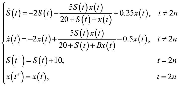 (18)
(18)
By calculating, we obtain

and
That is condition (5) holds. We choose initial value  = (1,1.3), (1,2.5), (3,3.4), (4,4.7), (5,6), (6,7.3), (7,7.9), (8,9.5), (9,10.7), (10,12.5) respectively, then from the numerical simulation (Figure 1) we see that there exists a positive periodic solution
  of system (18) such that any solution (S(t), x(t)) of system (20) with initial value
  tends to
  as
as . Therefore, if condition (5) holds, then system (18) has a positive periodic solution which is globally attracttive.
From Theorem 1, we consider dynamical behavior of the system (2) with D =1, a = 10, A = 10, B = 2, b = 1, k = 0.5, r = 0.2, p = 12, T = 2, then system (2) becomes
 (19)
(19)
By calculating, we obtain
 (a)
(a) (b)
(b)
Figure 1. (a) Time-series of the nutrient S for periodic oscillation; (b) Time-series of the microorganism population x for extinction.
and

That is condition (11) holds. We choose initial value  then from the numerical simulation (Figure 2) we see that system (19) is permanent.
It is difficult to study the global attractivity of system (2) analytically. We present here two examples to show that system (2) is global attractive under the condition (11). Setting D = 1, a = 6, A = 8, r = 0:4, p = 18, T = 2, b = 1, so that condition (11) holds. Choosing initial value  (2.5,1.6), (4.7,2.6), (7.1,6.3), (9.4,5.8), (12.2,7.3), (14.4), (16.5,9.7), (19.3,11.4), (21.4,12.5), (23,12), respectively, then from the numerical simulation (Figure 3) we see that there exist a unique T-period solution
  of system (2) which is globally attractive. Let D = 1, a = 6, A = 8, r = 0:2, p = 20, T = 2, b = 1. Then the condition (3.9) holds for those parameters. Choosing initial values
  = (0.5,0.4), (1,0.8), (1.5,1.2), (2,1.6), (2.5,2), (3,2.4), (3.5,2.8), (4,3.2), (4.5,3.6), (5,4), respectively, the numerical simulation (Figure 3) also show that system (2) is globally attractive. Therefore, we can guess if only condition (11) holds then
 (a)
(a) (b)
(b)
Figure 2. (a) Time-series of the nutrient S for permanence and periodic oscillation; (b) Time-series of the microorganism population x for permanence.
 (a)
(a) (b)
(b)
Figure 3. (a) Time-series of the nutrient S for global attractivity; (b) Time-series of the microorganism population x for global attractivity.
the system (2) has a unique T-period solution which is globally attractive
5. Acknowledgements
This work was supported by the National Natural Science Foundation of China (Grant Nos. 11261056, 11261058).
NOTES