Variable Selection for Partially Linear Varying Coefficient Transformation Models with Censored Data ()
1. Introduction
To model the effects of X on the failure time T, the following linear transformation models are considered
 , (1)
, (1)
where  is an unknown, strictly increasing function with
 ,
,  is a
is a  vector of unknown regression parameters, and the error term
  has a known continuous distribution that is independent of X. In the presence of censoring, we observe the event time
  and the censoring indicator
 , where C is the censoring time and
  is the indicator function. It is usually assumed that the censoring variable C is independent of T given X. Linear transformation model (1), encompassing Cox’s model and the proportional odds model as special cases, provide a popular tool in analyzing time-to-failure data, and have recently attracted considerable attention due to their high flexibility [1-4].
In practice, in order to accurately predict the survival time, many explanatory variables are generally collected and need to be assessed during the initial analysis. Deciding which covariates to have significant effect on the survival time and which variables are non-informative is practically interesting, but is always a tricky task for survival analysis. Variable selection is therefore of fundamental interest for survival analysis. Variable selection procedures for survival data have been studied extensively in the literature; see [5-7] for cox’s model; see [8] for proportional odds model.
Partially linear varying coefficient regression models have played an increasingly important role in statistical analysis for a good balance between flexibility and parsimony. Recently, varying coefficient regression models have been studied by many authors. [9] proposed a local least-squares method with a kernel weight function. [10] proposed an estimation procedure based on the local polynomial fitting method. [11] proposed a profile leastsquares technique for estimating the parametric components and applied the generalized likelihood ratio techniques to the testing problems for the nonparametric components. [12] proposed a class of efficient estimation method to estimate a partially linear varying coefficient model. Under quantile loss function, based on B-spline basis function approximations, [13] proposed the estimator and test for partially linear varying coefficient model. As for variable selection, [14] adopted the SCAD variable selection procedure to select important variables in the parametric components, and adopted the generalized likelihood ratio tests to select important variables in the nonparametric components of semi-parametric model. However, very little work has been done for partially linear varying coefficient transformation models with censored data, which are defined as following
 , (2)
, (2)
where  is an unknown, strictly increasing function with
 ,
,  comprises q unknown smooth functions,
  is a q dimensional covariate,
  is the regression parameters,
  is a p dimensional covariate, W ranges over a non-degenerate compact interval, without loss of generality, that is assumed to be the unit interval [0,1] and
  is the error with known continuous density,
  , and is independent of the covariates. In the absence of Z and W, model (2) reduces to a linear transformation model (1). When Z is a constant, model (2) reduces to a partial linear transformation model. [15] studied the partially linear transformation models using martingale representation based estimating equation. [16] proposed variable selection for the partially linear transformation models. To the best of our knowledge, there is no paper considering the variable selection for varying coefficient transformation models with censored data. To solve this problem, in this paper, we propose the penalized likelihood function method for variable selection in varying coefficient transformation models with censored data. The penalized likelihood function with adaptive Lasso is proposed. We only consider here the application of adaptive Lasso, because the convexity of
  penalty enables us to demonstrate the method easily. Nevertheless, the same idea is readily applicable to other shrinkage methods, such as SCAD proposed by [17], or one-step sparse estimator of [18]. The major advantages of the proposed procedures over the existing ones are their computational expediency and the most existing procedures are our special cases for survival data. Simulation experiments have provided evidence of the superiority of the proposed procedures.
The paper is organized as follows. In Section 2, we present the penalized maximum likelihood method with the adaptive Lasso (ALasso) penalty. A penalized maximum likelihood estimator is proposed for optimizing the penalized log marginal likelihood functions. In Section 3, we present an algorithm to implement the penalized maximum likelihood estimator. In Section 4, we conduct a simulation to detect the behavior of the proposed method. In Section 5, we illustrate the proposed procedure via analyzing lung cancer data.
2. Penalized Maximum Likelihood Estimation
Let  be independent and identically distributed copies of
 . The observations are
 . Thenfrom model (2), the log-likelihood function of
  can be written as
where  and
and  are the baseline and cumulative hazard functions of
 , respectively, and H is an increasing function. Throughout the paper,
  and
and  respectively denote the first and second derivatives of
  provided that they exist. Following [19] and [20], we approximate
  by the B-spline method.
Let  be a set of B-spline basis functions of order
  with
with  quasi-uniform internal knots. Then,
  can be approximated by
 , (3)
, (3)
where  is the spline coefficient vector, substituting (3) into the model (2), we can get log-likelihood function:

where .
.
In order to obtain the sparsity solution, this motivates us to consider a penalized log-likelihood function. The penalized log-likelihood function with adaptive Lasso is defined as
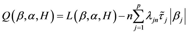 (4)
(4)
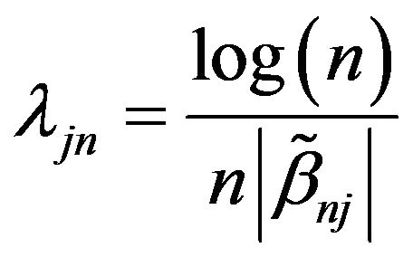
where  is tuning parameters. Denote the maximum likelihood estimate (MLE) as
 . Since
  are shown to be consistent [21]. Therefore, we choose
 .
.
3. Computation Algorithm
We provide an iterative computation algorithm to solve (4). In the spirit of nonparametric maximum likelihood, we restrict  to be a non-decreasing step function with
  and with jumps only at
 , where
  is the jth smallest observed failure time and
 is the total number of observed failures.
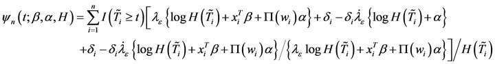
Consider

where  and
and  is
is  . A direct numerical maximization of the above
  may be problematic since the number of parameters,
  , may be very large. We recommend the following iteration procedure, which has been stable and effective in our numerical experience.
Step 1. Choose an intial value .
.
Step 2. Set the estimator to be  at the kth iteration. By differentiating
  with repect to
 , we can obtain
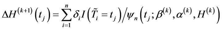
where
Then,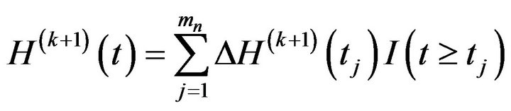 .
.
Step 3. By differentiating  with respect to
 , we obtain the score function,
  and obtain the root
  to the equation
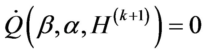 by using the Newton-Raphson iterative algorithm.
Step 4. Repeat Steps 2 and 3 until convergence.
4. Simulation Studies
In this section, we examine the finite sample performance of the proposed procedures. The model is
 , (6)
, (6)
where
 and the components of X is standard normal distribution. The correlation between
  and
and  is
is  with
with  and
and . Z is uniformly distributed on [0,2]. The distribution of W is independent of the Z and
 . The baseline hazard function of error
 is
is , where
  is constant; see [2]
and [21]. The model (6) reduces to the proportional hazards model if  and to the proportional odds model if
 . We consider
  and 1. The censoring time, C, follows the exponential distribution with mean 1. The largest follow-up time is set to 2.
In our simulation, we use the cubic B-spline with two interior knots to approximate the functional coefficient. The performance of  will be assessed by using the square root of average errors (RASE)
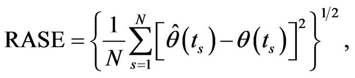
where  are the grid points at which the function
  is evaluated. In this simulation, N = 200 is used. To improve the computational efficiency, we choose
  by the method proposed by [22], which is
 , where
 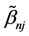 is maximum likelihood estimation without any penalty. To evaluate variable selection performance of adaptive Lasso and Oracle method, we report the results over 100 simulations in Table 1. Both columns “C” and “IC” are measures of model complexity. Column “C” shows the average number of zero coefficients correctly estimated to be zero, and column “IC” presents the average number of nonzero coefficients incorrectly estimated to be zero. As in [14], the performance of estimator
  will be assessed by using the generalized mean square error (GMSE), defined as
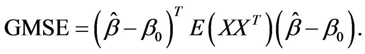
The column “GMSE” and “RASE” report both the mean of 100 GMSEs and RASEs, respectively.
We now summarize the main findings from Table 1.
1) The estimation errors of the ALasso method approach rapidly those of the oracle estimators as the sample size increases.
2) GMSE and RASE are decreasing with increase of sample size.
Figure 1 demonstrates the performance of the curve estimation of  for I with
 . From the Figure 1 we can see that the estimated curves are very close to the true curve
 . We may conclude that the proposed estimation of the function
  performs reasonably well. For other cases, the figures perform similarly with Figure 1, to save space, we omit them.
5. An Application
Now we illustrate the proposed procedures by an analysis of the lung cancer data from the Veteran’s Admini-
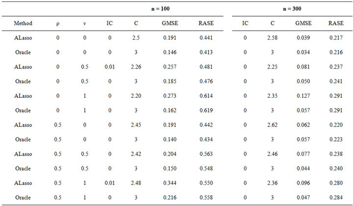
Table 1. Simulation results for different v, ρ and different sample size.

Figure 1. Estimated and curves (solid line) for v = 0 (dashdot line), and v = 1 (dash line). The left panel is the estimator of θ0(w) for ρ = 0. The right panel is the estimator of θ0(w) for ρ = 0.5.
stration lung cancer trail. In this trial, 137 males with advanced inoperable lung cancer were randomized to either a standard treatment or chemotherapy. Details of the study design and method have been given by [23]. The data set has been analyzed by many authors, for example, [5] fitted the proportional hazards model and [8] considered the proportional odds model. In both methods, all covariates were assumed linear, which may not be true, particularly for the age effect. It is well known that age is a complex confounding factor, and its effect usually shows a nonlinear trend [15].
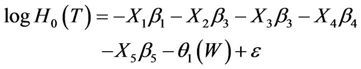
In our analysis, we take  to be the treatment: (1 = standard, 2 = test),
  to be cell type: (1 = squamous, 2
= small cell, 3 = adeno, 4 = large),  to be Karnofsky score,
  to be months from diagnosis,
  to be prior therapy (0 = no, 1 = yes) and W to be age. So we consider the following model:
 (7)
(7)
For estimation, we first rescale age between 0 and 1, and use cubic B-spline with two interior knots to approximate the nonparametric function as in simulations. We further apply the penalized likelihood function approach to select significant variable. For tuning parameters, we choose  by the method proposed by [22] as conducted in simulations. For comparison, we show the regression results for the proportional hazards model with
  and the proportional odds model with
 , respectively.
Table 2 gives estimators for the regression coefficient and corresponding standard errors. From Table 2, only the variable  is selected, in other words, only Karnofsky score has significant effect on survival time. Our findings is the same with [5] expect the age. Figure 2 gives the estimator of the nonlinear components. From Figure 2, it is easy to see that age has nonlinear effect on the survival function. Therefore, the partially linear transformation models can be more powerful in discovering significant covariates than those assuming simply linear covariate
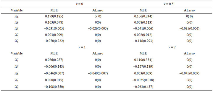
Table 2. Estimated coefficients for model (6).
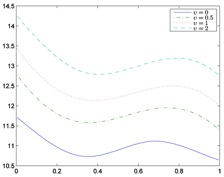
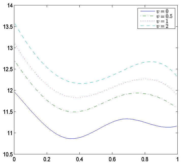
Figure 2. Estimated of  for v = 0, 0.5, 1 and 2.
effects, which is consistent with the conclusions of [16].
NOTES
#Corresponding author.