Optimality Conditions and Second-Order Duality for Nondifferentiable Multiobjective Continuous Programming Problems ()
1. Introduction
Second-order duality in mathematical programming has been extensively investigated in the literature. In [1], Chen formulated second order dual for a constrained variational problem and established various duality results under an involved invexity-like assumptions. Subsequently, Husain et al. [2], have presented Mond-Weir type second order duality for the problem of [1], by introducing continuous-time version of second-order invexity and generalized second-order invexity. Husain and Masoodi [3] formulated a Wolfe type dual for a nondifferentiable variational problem and proved usual duality theorems under second-order pseudoinvexity condition while Husain and Srivastav [4] presented a MondWeir type dual to the problem of [2] to study duality under second-order pseudo-invexity and second-order quasiinvexity.
The purpose of this research is to present multiobjective version of the nondifferentiable variational problems considered in [2,4] and study various duality in terms of efficient solutions. The relationship between these multiobjective variational problems and their static counterparts is established through problems with natural boundary values.
2. Definitions and Related Pre-Requisites
Let  be a real interval,
  and
and  be twice continuously differentiable functions. In order to consider
  where
where  is differentiable with derivative
 , denoted by
  and
and  the first order derivatives of
  with respect to
 and
and , respectively, that is,

Further denote by , and
, and  the
the  Hessian and
  Jacobian matrices respectively.
The symbols  and
and  have analogous representations.
Designate by X the space of piecewise smooth functions  with the norm
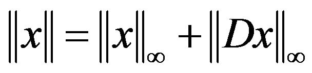 , where the differentiation operator D is given by

Thus  except at discontinuities.
We incorporate the following definitions which are required for the derivation of the duality results.
Definition 1. (Second-order Invex): If there exists a vector function  where
where  and with
  at
at  and
and  such that for a scalar function
 , the functional
  where
where  satisfies

then  is second-order invex with respect to
 where
where  and
and  the space of n-dimensional continuous vector functions.
Definition 2. (Second-order Pseudoinvex): If the functional  satisfies

then  is said to be second-order pseudoinvex with respect to
 .
.
Definition 3. (Second-order strict-pseudoinvex): If the functional  satisfies

then  is said to be second-order pseudoinvex with respect to
 .
.
Definition 4. (Second-order Quasi-invex): If the functional  satisfies
then  is said to be second-order quasi-invex with respect to
 .
.
Remark 1. If  does not depend explicitly on t, then the above definitions reduce to those for static cases.
The following inequality will also be required in the forthcoming analysis of the research:
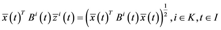
Lemma: 1 (Schwartz inequality): It states that

with equality in (1) if  for some
Throughout the analysis of this research, the following conventions for the inequalities will be used:
If  with
with  and
and
 , then

3. Statement of the Problem and Necessary Optimality Conditions
Consider the following nondifferentiable Multiobjective variational problem:
(VCP): Minimize

subject to
 (1)
(1)
 (2)
(2)

where 1)  denote the space of piecewise smooth functions x with norm
 , where differentiation operator D already defined.

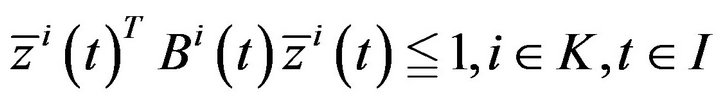
are assumed to be continuously differentiable functions, and 3) for each  is an
is an  positive semi definite (symmetric) matrix, with
  continuous on I.
In this section we will derive Fritz John and Karush-Kuhn-Tucker type necessary optimality conditions for (VCP).
Definition: A point  is said to be efficient solution of (VCP) if there exist
  such that

for some  and
and

for 
The following result which is a recast of a result of Chankong and Haimes [5] giving a linkage between an efficient solution of (VCP) and an optimal solution of p-single objective variational problem:
Proposition 1. (Chankong and Haimes [5]): A point  is an efficient solution of (VCP) if and only if
  is an optimal solution of
  for each
 : Minimize

subject to


for obtaining the optimal conditions for (VCP) we will use the optimal conditions obtained by Chandra et al. [6] for a single-objective variational problem which does not contain integral inequality constraints of .
.
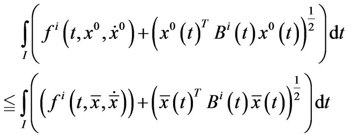
The validity of the following proposition is quite essential in obtaining the optimality conditions for (VCP)Proposition 2. If  is an efficient solution of (VCP), then
  is an optimal solution of the following problem
  for each
 : Minimize

subject to


Proof: Let  be an efficient solution of (VCP). Suppose that
  is not optimal solution of
 , for some
  Then there exists an
  such that

 (3)
(3)
and

The inequality (3) for 
 (4)
(4)
The inequalities (3) along with (4) contradicts the fact that  is an efficient solution of (VCP).
Hence  is an optimal solution of
 , for some
Theorem 1. (Fritz John Type necessary optimality condition): Let  be an efficient solution of (VCP). Then there exist
  and piecewise smooth functions
  and
and  such that
 (5)
(5)
 (6)
(6)
 (7)
(7)
 (8)
(8)
 (9)
(9)
Proof: Since  is an efficient solution of (VCP), by Proposition 2,
  is an efficient solution of
for each  and hence in particular
 . So by the results of [6] there exist
  and piecewise smooth functions
  and
and  such that


The above conditions yield the relations (5) to (9).
Theorem 2 (Kuhn-Tucker type necessary optimality condition):
Let  be an efficient solution of (VCP) and let for each
 , the conditions of
  satisfy Slaters or Robinson condition [6] at
 . Then there exist
  and piecewise smooth functions
  and
and 
 such that
 (10)
(10)
 (11)
(11)
 (12)
(12)
 (13)
(13)
 (14)
(14)
 (15)
(15)
Proof: Since  is an efficient solution of (VCP) by Proposition 2,
  is an optimal solution of
  for each
 . Since for each
 , the contradicts of
 , satisfy Slaters or Robinson conditions [6] at
 , by Kuhn-Tucker necessary condition of [6], for each
 , there exist
  and piecewise smooth function
  such that


Summing over  we obtain

where  for each
These can be written as,


where 
and 
Setting

we get


That is


4. Mond-Weir Type Second Order Duality
In this section, we present the following Mond-Weir type second-order dual to (VCP) and validate duality results:
(M-WD): Maximize

subject to
 (16)
(16)
 (17)
(17)
 (18)
(18)
 (19)
(19)
where

and

We denote by CP and CD the sets of feasible solutions to (VCP) and (M-WD) respectively.
Theorem 3. (Weak Duality): Assume that
(A1)  and
and
 .
.
(A2)  is second-order pseudoinvex.
(A3)  is second-order quasi-invex.
Then
 (20)
(20)
and
 (21)
(21)
cannot hold.
Proof. Suppose to the contrary, that (20) and (21) hold.
Since  we have

Since 
we have
Now, by the constraints (2), (18) and (19), we have

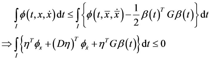
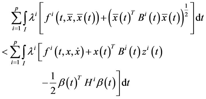
This by (A3), yields

By integration by parts, we have


This, by using (4) gives
 (22)
(22)


By hypothesis (A1), it implies
Using  in the above, we have

This contradicts (20) and (21). Hence the result.
Theorem 4 (Strong duality): Let  be normal and is an efficient solution of (VP). Then there exist
 , a piecewise smooth function
  such that
  is feasible for (M-WD) and the two objective functions are equal. Furthermore, if the hypotheses of Theorem 3 hold for all feasible solutions of (VCP) and (M-WD) ,then
  is an efficient solution of (M-WD).
Proof: Since  is normal and an efficient solution of (VP), by Proposition 2, there exist
  and piecewise smooth
  and
and  satisfying
 (23)
(23)
 (24)
(24)
 (25)
(25)
 (26)
(26)
 (27)
(27)
From (24) along with , we have

Hence

satisfies the constraints of (M-WD) and
That is, the two objective functionals have the same value.
Suppose that  is not the efficient solution of (M-WD). Then there exists
  such that

As , we have

This contradicts the conclusion of Theorem 3. Hence  is an efficient solution of (M-WD).
Theorem 5 (Converse duality):
(A1): Assume that  is an efficient solution of (M-WD)
(A2): The vectors  are linearly independent where
  the
the  row of is
  and
and  is the
  row of G,
(A3)
are linearly independent and
(A4) for  either a)
and 
or b) 
and 
Then  is feasible for (VCP) and the two objective functionals have the same value. Also, if Theorem 3 holds for all feasible solutions of (CP) and (M-WD), the
  is an efficient solution of (VCP).
Proof: Since  is an efficient solution of (M-WD), there exist
 ,
,  and
and , and piecewise smooth
 ,
,  ,
,  and
and  such that the following Fritz John optimality conditions (Theorem 1)
 (28)
(28)
 (29)
(29)
 (30)
(30)
 (31)
(31)
 (32)
(32)
 (33)
(33)
 (34)
(34)
 (35)
(35)
 (36)
(36)
 (37)
(37)
 (38)
(38)
From (31), we have
 (39)
(39)
This, by the hypothesis (A2) gives
 (40)
(40)
and  (41)
(41)
Using (40), (41) and (17), we have
 (42)
(42)
Let  Then (41) gives
  and (40) gives
 ,
, 
Using  and
and , (42) implies

This, because of (A3) yields
 (43)
(43)
The relation (43) with  gives
gives 
Since , (36) gives
  The relation (30) yields
  we have
 ,
,  from (32) and
 ,
,  ,
,  from (35). These yield
 ,
,  ,
, .
.
Consequently

contradicting (38).
Hence  and from (43)
Multiplying (30) by , summing over j, and then using (34) and (41), we have

In view of the hypothesis (A4), this gives ,
,
 , The relation (30) implies
 ,
,
 yielding the feasibility of
  for (VCP).
The relation (32) with  and
and  gives
gives
 (44)
(44)
This by Schwartz inequality gives
 (45)
(45)
If  then (35) give
 ,
, . and so (45 ) implies
If  (44) gives
 . So we still get

Now suppose that  is not an efficient of (VCP). Then, there exists
  such that

and

Using  and
and

We have

for some  and
and

This contradicts Theorem 3. Hence  is an efficient solution for (VCP).
Theorem 6 (Strict converse duality): Assume that
is second-order strictly pseudoinvex, and
 is second-order quasi-invex with respect to same
 . Assume also that (VCP) has an optimal solution
  which is normal [6]. If
  is an optimal solution of (M-WD), then
  is an efficient solution of (VCP) with
Proof: We assume that  and exhibit a contradiction. Since
  is an efficient solution, it follows from Theorem, that there exist
 ,
,  ,
,  ,
,  ,
,  ,
,  and
and  such that

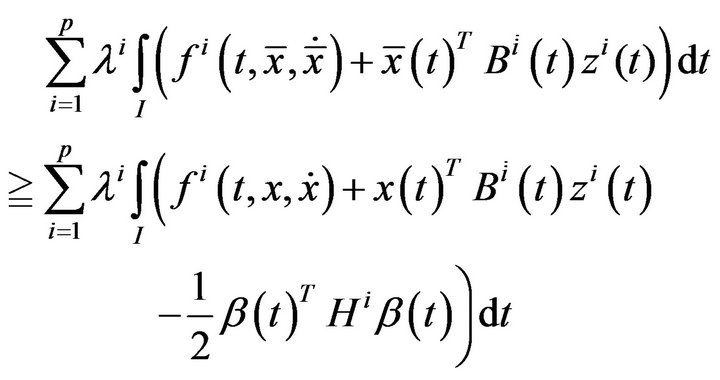
is an efficient solution of (M-WD). Since  is an optimal solution of (M-WD), it follows that

This, because of second-order strict-pseudoinvexity of
 (46)
(46)
Also from the constraint of (VCP) and (M-WD), we have
Because of second-order quasi-invexity of
 , this implies
 (47)
(47)
Combining (46) and (47), we have

(By integrating by parts)
This, by using η = 0, at t = a and t = b, implies

contradicting the feasibility of
 for (M-WD).
5. Problems with Natural Boundary Values
In this section, we formulate a pair of nondifferentiable Mond-Weir type dual variational problems with natural boundary values rather than fixed end points given bellow
 : Minimize

Subject to

 : Maximize

Subject to


 and
and , at
, at .
.

We shall not repeat the proofs of Theorems 3-6 for the above problems, as these follow on the lines of the analysis of the preceding section with slight modifications.
6. Non-Linear Multiobjective Programming Problem
If the time dependency of  and
and  is ignored, then these problems reduce to the following nondifferentiable second-order nonlinear problems already studied in the literature:
(VP1): Minimize

subject to

(VD1): Maximize

subject to

NOTES