Non-Linear Mathematical Model of the Interaction between Tumor and Oncolytic Viruses ()
1. Introduction
Oncolytic viruses are viruses that infect and kill cancer cells but not normal cells [1-4]. Oncolytic virus therapy originated early in the last century upon the observation of occasional tumor regressions in cancer patients suffering from virus infections or those receiving vaccinations. Many types of oncolytic viruses have been studied as candidate therapeutic agents including adenoviruses, herpes viruses, reoviruses, paramyxoviruses, retroviruses, and others [2,4]. Probably, the best-characterized oncolytic virus, that has drawn a lot of attention, is ONYX- 015, an attenuated adenovirus that selectively infects tumor cells with a defect in the p53 gene [3]. This virus has been shown to possess significant antitumor activity and has proven relatively effective at reducing or eliminating tumors in clinical trials [5-7]. Furthermore, a small number of patients who were treated with the oncolytic virus showed regression of metastases [2]. Although safety and efficacy remain substantial concerns, several other oncolytic viruses acting on different principles, including tumor-specific transcription of the viral genome, have been developed, and some of these viruses have entered in trials [2,8-10].
The oncolytic effect has several possible mechanisms that yield complex results. The first such mechanism is the result of viral replication within the cell and rupture out of the cell [11,12]. The third mechanism involves virus infection of cancer cells that induces antitumoral immunity. Surviving mice acquired a resistance to rechallenge with tumor cells [13]. Host immune response maximizes antitumor immunity but also interferes with virus propagation. Wakimoto et al. [14] studied the limitation of virus propagation caused by host immune response in the central nervous system. Ikeda et al. [15] showed that the viral survival term was prolonged and that virus propagation was increased by the anti-immune drug, cyclophosphamide.
Several mathematical models that describe the evolution of tumors under viral injection were recently developed. Wodarz [13,16] presented a mathematical model that describes interaction between two types of tumor cells (the cells that are infected by the virus and the cells that are not infected by the virus) and the immune system. However, to the best of our knowledge, till date no general analytical expressions for the mathematical modeling of two populations of cells namely uninfected tumor cells and infected cells [17]. The purpose of this paper is to derive approximate analytical expression of two types of cells growing namely uninfected and infected tumor cells by solving the non-linear differential equations using Homotopy analysis method [18-20].
2. Mathematical Models
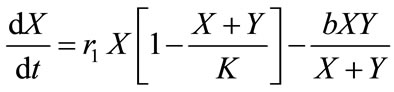
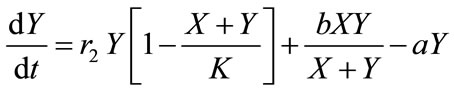
The model, which considers two types of cells growing in the logistic fashion, has the following form [17]:
 , (1)
, (1)
 (2)
(2)
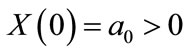
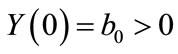
The equation can be solved subject to the following initial conditions:
 (3)
(3)
 (4)
(4)
where X is the size of the uninfected cell population; Y is the size of the infected cell population;  and
and  are the maximum per capita growth rates of uninfected and infected cells; K is the carrying capacity; b is the transmission coefficient; and a is the rate of infected cell killing by virus. We introduce the following set of dimensionless variables as follows [17]:
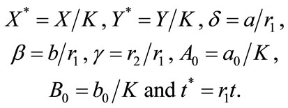 (5)
(5)
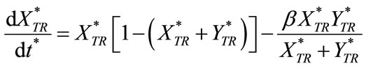
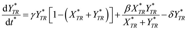
The governing non-linear differential equations (Equations (1) and (2)) expressed in the following non-dimensionless format:
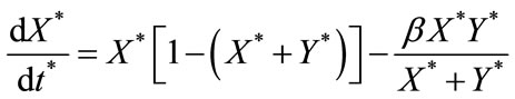 (6)
(6)
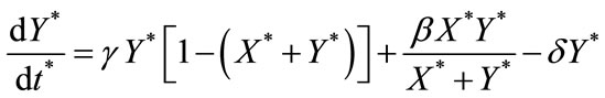 (7)
(7)
An appropriate set of boundary condition are given by:
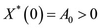 ,
, (8)
(8)
3. Solution of Boundary Value Problem Using Homotopy Analysis Method
The Homotopy analysis method (HAM) is a powerful and easy-to-use analytic tool for nonlinear problems [21- 23]. It contains the auxiliary parameter h, which provides us with a simple way to adjust and control the convergence region of solution series. Furthermore, the obtained result is of high accuracy. Solving the Equations (6) and (7) using HAM (see Appendix A) and simultaneous equation method (see Appendix B and C), the steady state and transient contributions to the model are given by:
 (9)
(9)
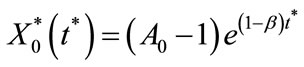
where
 (10)
(10)
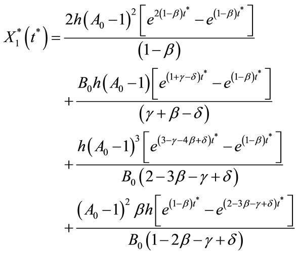
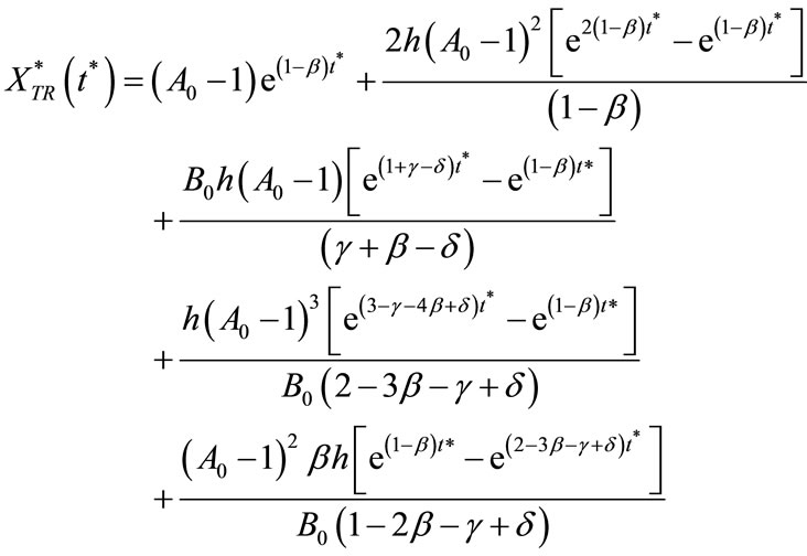 (11)
(11)
Similarly we can obtain  as follows:
 (12)
(12)
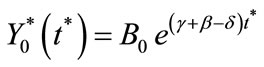
where
 (13)
(13)
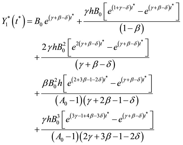
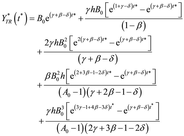 (14)
(14)
Here  and
and  represent a time independent steady state term and
  and
and  denote the time dependent transient component. The steady state term will be important at long times as
  In contrast the transient term will be of important at short times as
4. Numerical Simulation
The non-linear equations (Equations (6) and (7)) for the boundary conditions (Equation (8)) are solved by numerically. The function ode45 in Scilab software is used to solve two-point boundary value problems (BVPs) for ordinary differential equations. The Matlab program is also given in Appendix C. The numerical results are also compared with the obtained analytical expressions (Equations (9) and (12)) for all values of parameters ,
,  ,
,  ,
,  and
and .
.
5. Results and Discussion
Equations (9) and (12) represent the simple approximate analytical expressions of the uninfected and infected tumor cells for all values of parameters ,
,  ,
,  ,
,  and
and . The two types of tumor cell growing using Equations (9) and (12) are represented in Figures 1-4. In Figures 1 and 2, the dimensionless uninfected tumor cells reach the constant value when
  for some fixed value of
  and different values of
  and
and . The dimensionless infected tumor cells
  reaches the
steady state value when .
.
In Figures 3 and 4, the dimensionless infected tumor cells reach the constant value when  for some fixed value of
  and different values of
  and
and . The dimensionless infected tumor cells
  reaches the steady state value when
 . Figures 5 and 6 give us the confirmation for the above discussion in three-dimensional graphs also.

Figure 5. The normalized three-dimensional of dimensionless uninfected tumor cells X*(t*) (Equation (9)) for t* = 0 to 1.
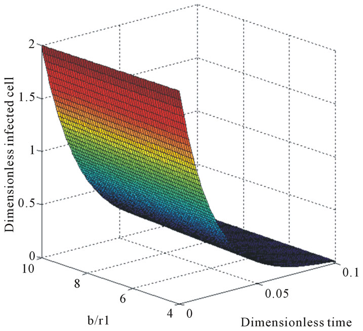
Figure 6. The normalized three-dimensional of dimensionless infected tumor cells Y*(t*) (Equation (12)) for t* = 0 to 0.1.
6. Conclusion
In this work, the coupled system of time dependent differential equations for the two types of cells growing has been solved analytically using the Homotopy Analysis Method. Approximate analytical expressions for uninfected and infected cell population are derived for all values of parameters. Furthermore, on the basis of the outcome of this work, it is possible to calculate the approximate rate of the tumor cells growth. The extension of the procedure to other systems that include interaction between tumor cells and anticancer agents seem possible.
7. Acknowledgements
This work was supported by the Council of Scientific and Industrial Research (CSIR No.: 01(2442)/10/EMR-II), Government of India. The authors also thank Mr. M.S. Meenakshisundaram, Secretary, The Madura College Board, Dr. R. Murali, The Principal, and Prof. S. Thigarajan, HOD, Department of Mathematics, The Madura College, Madurai, Tamilnadu, India for their constant encouragement. The authors S. Usha is very thankful to the Manonmaniam Sundaranar University, Tirunelveli for allowing the research work.
Appendix A: Basic Concept of Liao’s Homotopy Analysis Method (HAM)
Consider the following nonlinear differential equation
 (A1)
(A1)
where N is a nonlinear operator, t denotes an independent variable,  is an unknown function. For simplicity, we ignore all boundary or initial conditions, which can be treated in the similar way. By means of generalizing the conventional Homotopy method, Liao constructed the so-called zero-order deformation equation as:
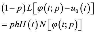 (A2)
(A2)
where  is the embedding parameter,
  is a nonzero auxiliary parameter,
  is an auxiliary function, L is an auxiliary linear operator,
  is an initial guess of
 ,
,  is an unknown function. It is important, that one has great freedom to choose auxiliary unknowns in HAM. Obviously, when
  and
and , it holds:
 and
and  (A3)
(A3)
respectively. Thus, as p increases from 0 to 1, the solution  varies from the initial guess
  to the solution
 . Expanding
  in Taylor series with respect to p, we have:
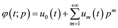 (A4)
(A4)
where
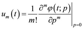 (A5)
(A5)
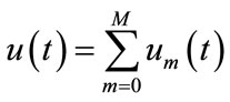
If the auxiliary linear operator, the initial guess, the auxiliary parameter h, and the auxiliary function are so properly chosen, the series (A4) converges at p = 1 then we have:
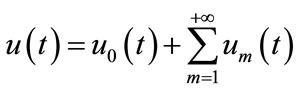 . (A6)
Define the vector
 (A7)
(A7)
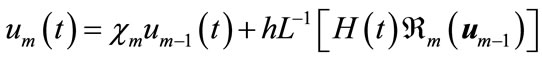
Differentiating Equation (A2) for m times with respect to the embedding parameter p, and then setting  and finally dividing them by m!, we will have the socalled mth-order deformation equation as:
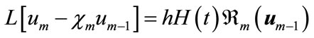 (A8)
(A8)
where
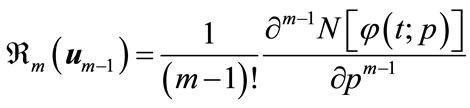 (A9)
(A9)
and
 (A10)
(A10)
Applying  on both side of Equation (A8), we get
 (A11)
(A11)
In this way, it is easily to obtain  for
for  at
at  order, we have
 (A12)
(A12)
When , we get an accurate approximation of the original Equation (A1). For the convergence of the above method we refer the reader to Liao. If Equation (A1) admits unique solution, then this method will produce the unique solution. If Equation (A1) does not possess unique solution, the HAM will give a solution among many other (possible) solutions.
Appendix B: Steady State Solution
For the case of steady-state condition, the Equations (6) and (7) becomes as follows:
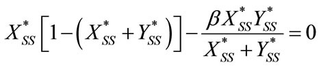 (B1)
(B1)
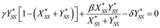 (B2)
(B2)
Solving the above Equations (B1) and (B2), we get
 (B3)
(B3)
and
 . (B4)
Thus we can obtain  and
and  as in the text (Equations (10) and (13)).
Appendix C: Non-Steady State Solution of the Equations Using the HAM
The given differential equations for the non-steady state condition are of the form as:
 (C1)
(C1)
 (C2)
(C2)
For the transient part, the initial conditions are redefined as
 (C3)
(C3)
 (C4)
(C4)
In order to solve the Equations (C1) and (C2) by means of the HAM, we first construct the Zeroth-order deformation equation by taking ,
,
 (C5)
(C5)
 (C6)
(C6)
We have the solution series as
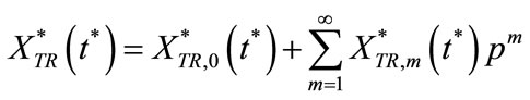 (C7)
(C7)
and
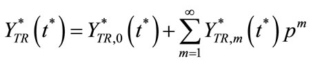 (C8)
(C8)
where
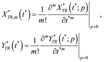 (C9)
(C9)
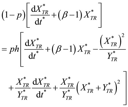
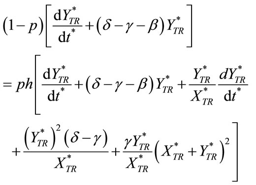
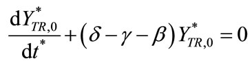
Substituting Equations (C7) and (C8) into Equations (C5) and (C6) and comparing the coefficient of like powers of p, we get
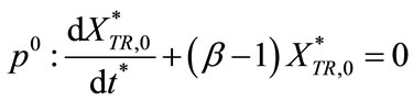 (C10)
(C10)
 (C11)
(C11)
 (C12)
(C12)
 (C13)
(C13)
and so on.
The initial conditions are redefined as
 (C14)
(C14)
 (C15)
(C15)
and
 for
for  (C16)
(C16)
Solving the Equations (C10) and (C10) by using the boundary conditions given in Equations (C14) and (C15), we get
 (C17)
(C17)
and
 (C18)
(C18)
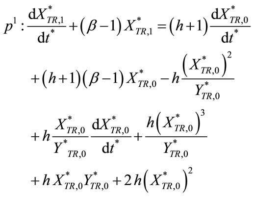
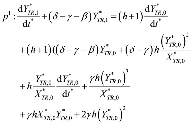
Substituting the Equations (C17) and (C18) in Equations (C12) and (C12) and by using the boundary conditions given in Equation (C16), we get
 (C19)
(C19)
and
 (C20)
(C20)
Adding the Equations (C17) and (C19) and the Equations (C18) and (C20), we get the Equations (9) and (12) as in the text.
Appendix D: MATLAB Program to Find the Numerical Solution of Non-Linear Equations (6) and (7)
function main1 options= odeset('RelTol',1e-6,'Stats','on');
Xo = [10; 2];
tspan = [0,10];
tic
[t,X] = ode45(@TestFunction,tspan,Xo,options);
toc figure hold on plot(t, X(:,1),'blue')
plot(t, X(:,2),'green')
return function [dx_dt]= TestFunction(t,x)
a=16;
b=3;
r=10;
dx_dt(1) =x(1)*(1-(x(1)+x(2)))-(b*x(1)*x(2))/(x(1)+x(2));
dx_dt(2)=r*x(2)*(1-(x(1)+x(2)))+(b*x(1)*x(2))/(x(1)+x(2))-a*x(2);
dx_dt = dx_dt';
Appendix E: Nomenclature
Symbol Meaning
 Size of the uninfected cell population
 Size of the infected cell population
 Rate of infected cell killing by the virus
 Transmission coefficient
 Maximum per capita growth rates of uninfected cells
 Maximum per capita growth rates of infected cells
 Carrying capacity
 Time
Time
 Size of the dimensionless uninfected cell population
 Size of the dimensionless infected cell population
 Dimensionless time