Distributed Alternating Direction Method of Multipliers for Multi-Objective Optimization ()
1. Introduction
In the network age, there exist a variety of network systems, such as communication network system, transportation network system, power network system and sensor network system. These network systems are usually called multi-agent systems. A multi-agent system is a large-scale network system associated with multiple agents. In the multi-agent system, each individual with communication, computing, perception, decision-making, learning and execution abilities is called an agent, also known as a node in the network topology. In a broad sense, agents can be a robot, an aircraft, a computer and other entities, which can interact with each other through network connections and cooperate to complete some complex tasks.
Many optimization problems encountered in multi-agent systems, such as the cyber-physical social system [1], classification [2], task scheduling [3] and energy system [4], often involve multiple conflicting objectives. This kind of optimization problem is called Multi-Objective Optimization Problem (MOP).
There are many ways to solve multi-objective optimization problems, which can be divided into three types: scalarization methods, classical optimization algorithms and intelligent algorithms. Scalarization methods transform complex multi-objective optimization problems into single-objective optimization problems, containing the main objective method, linear weighting method, minimax method, ideal point method and so on [5]. Classical optimization algorithms extend the algorithms for solving single-objective optimization problems to multi-objective optimization problems, including steepest descent method [6], Newton method [7] [8], proximal point method [9] [10], projected gradient method [11] [12] and penalty-type function method [13]. Intelligent algorithms include the genetic algorithm [14], evolutionary algorithm [15] [16] and so on.
Among these methods, scalarization methods are widely used because their models are easy to understand and relatively easy to solve. Among them, the linear weighting method is one of the commonly used approaches to solve multi-objective optimization problems. It can also coordinate the preference settings of multiple targets, which increases the subjectivity factor to some extent.
Most of the above optimization algorithms are centralized, and such methods need a central node to collect data and calculate the optimal decision. For example, in the electric-gas integrated energy system, a joint control center should be introduced as the decision-making mechanism for unified control of the electric-gas coupling system. Therefore, the communication burden and computation cost of the central node are high, and its scalability, robustness and adaptability are poor [17]. In contrast, distributed optimization algorithms are a kind of decentralized algorithms, which only require the network to be a general-connected graph, but do not need the central node. They decompose a large optimization problem into several sub-problems and compute each sub-problem, so as to optimize the original problem. Therefore, distributed optimization algorithms have high computational efficiency, small communication volume and strong reliability [18].
There are many distributed algorithms, including discrete algorithms and continuous algorithms [19] [20] [21] [22]. Among them, the discrete distributed algorithms can be divided into two kinds. The first one is the original algorithm [23] [24] [25], which weighted averages local estimates with neighboring states to make local states consistent. One of the great advantages of these methods is that they require less computation, but their convergence speed is slow and their accuracy is relatively low. The other is the dual algorithm that includes the augmented Lagrange method [26] and Alternating Direction Method of Multipliers (ADMM) [27] - [32]. Because each node needs to solve a sub-problem, the dual algorithm usually requires a relatively large amount of computation, but they can quickly converge to the exact optimal solution.
As an important method of distributed optimization algorithm, the alternating direction multiplier method has the characteristics of protecting data privacy and fast convergence. It has been shown that even for non-smooth and non-convex cost functions, the alternating direction multiplier method can achieve satisfactory convergence speed [33]. In addition, it is robust to noise and error [34].
Based on the above reasons, this paper proposes a distributed alternating direction method of multipliers to solve a class of multi-objective optimization problems in multi-agent systems. This algorithm does not need the central node, and thus it can effectively avoid the shortcomings of the centralized algorithms. As a result, the algorithm proposed in this paper has the characteristics of low communication cost, strong privacy, fast convergence and so on.
The rest of this paper is organized as follows. In Section 2, a multi-objective optimization problem is introduced and it is transformed into a single-objective optimization problem. Based on this single-optimization objective problem, a distributed ADMM algorithm is proposed in Section 3. In Section 4, numerical experiments are provided to verify the effectiveness of the proposed algorithm. Finally, the conclusions of this paper are presented in Section 5.
2. Problem Model
This paper studies the following multi-objective optimization problem:
(1)
where
is the global optimization variable, n is the number of agents in the multi-agent system and
is a convex local cost function. Each
is known only by agent i and the agents cooperatively solve the multi-objective optimization problem.
The network topology of the multi-agent system is assumed to be a general undirected connected graph, which is described as
, where V denotes the set of agents,E denotes the set of the edges and
,
. These agents are arranged from 1 to n. Edges between i and j with
are represented by
or
and
means that agents i and j can exchange data with each other. The neighbors of agent i are denoted by
and
.
The edge-node incidence matrix of the network G is denoted by
. The row in A that corresponds to the edge
is denote by
, which is defined by:
Here, the edges of the network are sorted by the order of their corresponding agents. For instance, the edge-node incidence matrix of the network G in Figure 1 is given by:
According to the edge-node incidence matrix, the extended edge-node incidence matrix A of the network G is given by:
where
denotes the Kronecker product. Obviously, A is a block matrix with
blocks of
matrix.
By introducing separating decision variable
for each agent
, problem (1) has the following form:
(2)
where
. Clearly, the problem (2) is equivalent to problem (1) if G is connected.
With the help of the extended edge-node incidence matrix A, the problem (2) can be rewritten in the following compact form:
(3)
Denote the feasible region of problem (3) by
, and thus the definition of effective solution (or weak effective solution) to problem (3) is given below.
Definition 2.1. [5] If there does not exist
, such as
(or
), where
, then
is the effective solution (or weak effective solution) of problem (3). Here,
and
are taken element-wise.
In order to solve the multi-objective optimization problem by alternating direction multiplier method, it needs to be transformed into a single-objective optimization problem. By the linear weighting method, the single-objective optimization problem of problem (3) is constructed as follows:
(4)
Here,
or
, where:
Remark 2.1. [5] For each given
(or
), the optimal solution of problem (4) must be a efficient (or weakly efficient) solution to problem (3).
Denote
,
, then problem (4) can be rewritten as:
(5)
Remark 2.2. According to the convexity of
, each component
of
is a convex function, and thus
is also convex.
3. Algorithm Design
The augmented Lagrangian function of problem (5) is defined by:
(6)
where
is the penalty parameter of the constraint
and
. The Jacobi-Proximal ADMM algorithm for problem (5) is designed as follows:
(7)
(8)
where the proximal matrix P is a block diagonal matrix and
. Combining the linear and quadratic terms of the augmented Lagrangian function, (7) can be rewritten as:
(9)
Denoting the block corresponding to the agenti by
, one can rewrite (9) in the following form:
(10)
It is worth noting that each row of the constraint
corresponds to one edge
in the set E. Hence, one has
for any
, where
. Denote the multiplier corresponding to the edge
by
. Then, the iteration of x can be refined as:
(11)
Thus, the iteration of x have the following distributed version:
(12)
Similarly, by the characteristic of matrix A, (8) can be rewritten as:
(13)
Therefore, the iterations of the multipliers are also distributed to the agents.
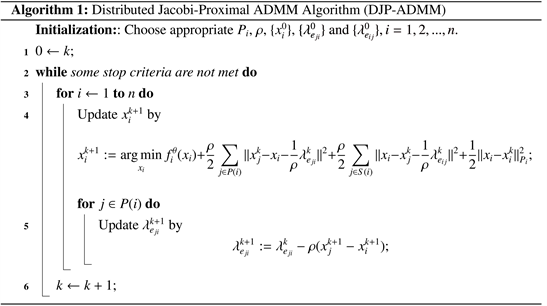
The distributed Jacobi-Proximal ADMM algorithm for problem (5) is described as Algorithm 1.
4. Numerical Experiment
Consider the following multi-objective optimization problem:
(14)
where
,
,
and
. Obviously, the solutions to these two objective functions are
and
, respectively. By the convexity of these functions, the weak
efficient solution of problem (14) is
and its efficient solution is
if
.
Assume the connected network
with n agents and m edges. Each edge is generated randomly. The connectivity ratio of the network G is denoted
by
. The multi-objective optimization problem (14) can be reformulated into a distributed version:
(15)
where
.
By linearly weighting the objective functions, problem (15) can be transformed into the following single-objective optimization problem:
(16)
where A is the extended edge-node incidence matrix of the network G,
and
is convex. Therefore, Algorithm 1 can be used to solve problem (16).
The proximal matrix of Algorithm 1 is set by
. In this case, the iteration of x has a closed-form solution, which is shown as follows:
where
is the number of neighbors of the agent i.
To verify the effectiveness of Algorithm 1, we generate a network with
nodes and
. The network generated is shown as Figure 2. The value of the parameters are set as:
and
. The graph of the two objective functions is shown as Figure 3. Obviously, the weak efficient solution is
and the efficient solution is
.
![]()
Figure 3. The graph of the two objective functions.
![]()
Table 1. Different weights and solutions to the corresponding problems.
![]()
![]()
Figure 4. The graph of the objective function and the solutions of problem (16).
Different weights are selected, and then Algorithm 1 is used to solve the corresponding single-objective problem (16). The results obtained are shown in Table 1. Besides, the graph of the objective function and the solutions of problem (16) is shown as Figure 4.
5. Conclusions
In this paper, a distributed ADMM algorithm is put forward to solve a kind of multi-objective optimization problem. This algorithm does not need the central node, and thus its communication cost is low and privacy is high. In addition, the effectiveness of the algorithm is verified by some numerical experiments.
There are a few distributed algorithms for multi-objective optimization problems. The method adopted in this paper is to transform the multi-objective optimization problem into a single-objective optimization problem through the linear weighting method, and then solve this single objective optimization problem, instead of solving the multi-objective optimization problem directly. Therefore, it is a challenge to design a distributed algorithm for directly solving multi-objective optimization problems and to verify its convergence, which is also worth exploring.