Elastic Full Waveform Inversion Based on the Trust Region Strategy ()
1. Introduction
The physical properties of the earth can be inverted quantitatively by the reflected seismic waves. In modern seismology, traveltime inversion is the main technique approach in the 19th century. Since the 1980s [1] [2], full waveform inversion (FWI) has become a rapidly developing subject because of its high resolution for reconstructing media parameters.
In FWI, the Fréchet derivative is required to estimate explicitly before proceeding to the inversion of the linearized system [3]. However, the computational cost of calculating Fréchet or gradient is too large. So some other methods have been taken into account. In [1] [2], the authors proposed to compute the gradient by solving an adjoint problem, which is considered as the initial of time-domain FWI. Since then, the FWI has been an important research topic in exploration geophysics. In the 1990s, the time-domain FWI was extended to the frequency domain [4] [5]. The frequency-domain FWI has the advantage of high computational efficiency and flexibility of data selection [6].
The FWI is actually an optimization iterative process to solve a nonlinear optimization problem. Generally, the computational cost of global optimization methods is extensive large. For this reason, local optimization algorithms are adopted. To avoid iteration falling to an unreasonable local minimum point, the multiscale method was proposed [7] in 1995. The multiscale method performs the inversion from the low frequency to high-frequency information step by step. It includes the long-wavelength information of the model and thus it enhances the robustness of inversion effectively. It can overcome the problem of local minima caused by the poor initial model selection. This technique has been successfully applied to the time-domain acoustic FWI, see e.g. [8] [9]. In order to reconstruct the long wavelength of the macroscopic velocity model, the Laplace-domain FWI is proposed [10]. A hybrid domain method combining the Laplace-domain method and the frequency-domain method together is also developed [11]. This method can be regarded as a special case of frequency-domain damping inversion.
In elastic FWI, there are three different parameters, i.e., density and two Lamé parameters. In [12], the authors pointed out that different parameters have coupled effects on the seismic response which is called the trade-off effect or crosstalk. In order to tame the trade-off effect, several hierarchical inversion strategies are developed. In [13], Lamé parameters are inverted with fixed density first and then velocities are updated. In [14], all parameters are inverted simultaneously. However, the overall steplength is estimated by calculating an optimal steplength for every parameter individually.
The Hessian matrix plays an important role in FWI. It contains the information of multiple scattering wavefields and the trade-off effects among different parameters. The off-diagonal blocks of Hessian reflect the relationship between different parameters [12]. The Newton-type method such as the quasi-Newton method, the Gauss-Newton method [15] and the truncated Newton method [16] all contain the Hessian information and so they behave better than the steepest descent method in accuracy. In the calculation of the gradient vector, the adjoint method is usually used [17]. The adjoint method can be extended to the truncated Newton method [18]. For the elastic wave equations, the wave propagator operator is symmetric. The back propagator operator and the forward propagator operator are identical. Besides that, the Gauss-Newton approximation of Hessian matrix is positive and definite. This property can be used in the trust region strategy. Our investigations in this paper show that the trust region method can accelerate the convergence rate and improve the inversion accuracy.
In this paper, we investigate the application of the trust region strategy in FWI. The rest of our paper is organized as follows. In Section 2, the theoretical methods are described in detail. In Section 3, numerical computations and comparisons are presented. Finally, in Section 4, the conclusion is given.
2. Theory
In this section, we will introduce the forward problem first. Then we will describe FWI based on the trust region method. In order to solve the subproblem in the trust region algorithm, the two dimensional subspace method is described.
2.1. Forward Method
The source-free time-domain two dimensional (2D) elastic wave equations can be written as [19]
(2.1)
(2.2)
where
is the density,
and
are the Lamé parameters,
and
are the displacement in the horizontal
and vertical
directions respectively. Furthermore, (2.1) and (2.2) can be rewritten as the following stress-velocity formulation after adding a source
(2.3)
where
and
are the particle velocity components in the
and
directions respectively,
,
,
are the stress tensor components. Here we have added the source, i.e., the body force
and
vector to
and
components respectively. We rewrite the system (2.3) in the following matrix form
(2.4)
(2.5)
where
,
,
denote
,
,
. The symbol
denotes the adjoint
operator. Note that the determinant of the matrix C is positive. So from (2.4) and (2.5), we have
(2.6)
The compact form of the forward problem is
(2.7)
where
is the model parameters,
. In (2.7), the wave propagator
is symmetric. Given the media parameters
,
and
, the forward problem is to solve system (2.6) numerically.
We have many numerical methods to solve system (2.6), for example, the finite volume method [20] and the staggered-grid method [21] and so on. In this paper, we use the staggered-grid method for its high computational efficiency and relatively easy code implementation. Since the computational domain is finite, the absorbing boundary conditions [22] are required to absorb the boundary reflections. In this paper, we adopt the perfectly matched layer (PML) method [23] [24]. The forward discrete schemes for solving system (2.3) are given in Appendix A.
2.2. Full Waveform Inversion
The FWI is a data-fitting procedure to find the model parameter
by minimizing the data misfit
between the simulated data
and the observed data
. The objective function can be formulated as
(2.8)
where T is the total recording duration,
and
are the number of the sources and receivers respectively. Once the media parameters
,
, and
are inverted, we can yield the P-wave velocity and S-wave velocity by
(2.9)
respectively.
The misfit function
is minimized iteratively. The update procedure in FWI at
-th iteration can be expressed as
(2.10)
where
and
are the model parameter at
and
iteration respectively,
denotes the step length at
iteration,
is the descent direction. The step length
must be found by using the line search technique for nonlinear inverse problem.
Neglecting the summation in (2.8) and introducing the restriction operator R at receiver points, then the gradient of the objective function with respect to the model parameter
is
(2.11)
where
is the adjoint operator. Furthermore, the Hessian matrix can be obtained by taking derivative of (2.11) with respect to the model parameter
(2.12)
The expression of Hessian H is divided into two parts, i.e.,
and
. The first part
is the Gauss-Newton approximation of Hessian [15], which just contains the 1st-order derivative of the wavefield. The second part
contains the 2nd-order derivative of the wavefield. The full Newton method consists of both the parts
and
[15]. The truncated Newton is based on the computations of descent direction by the conjugated gradient algorithm in the full Newton framework. The BFGS method is an efficient algorithm to compute the inverse of Hessian approximation in the Gauss-Newton method. It is the first quasi-Newton algorithm and named for its discovers Broyden, Fletcher, Goldfarb and Shanno. To save storage memory further, the limited-memory BFGS (L-BFGS) algorithm is usually applied [25] [26] [27] in computations.
2.3. Gradient Calculation
The gradient of the objective function can be obtained by the Lagrangian formulation [17] [18] [28] or the perturbation theory [29]. Following the perturbation theory [29], the gradient of the objective function with respect to model parameters can be rewritten as
(2.13)
(2.14)
(2.15)
where
and
are the forward displacements in the
and
directions respectively, and
and
are the corresponding backward displacements in the
and
directions respectively. Equations (2.13)-(2.15) are the gradient expressions in terms of the displacements.
We solve the forward problem based on (2.3) instead of (2.1)-(2.2) by the staggered-grid method. So it is necessary to express the gradient (2.13)-(2.15) with the particle velocity and the stress tensor. The results are the following
(2.16)
(2.17)
(2.18)
where
,
,
,
,
are the solutions of forward problem (2.3) whereas
,
,
,
and
are the solutions of corresponding adjoint problem. The derivation is given in Appendix B.
2.4. Trust Region Method
There are two strategies to solve a minimization problem. One is the line search method and the other is the trust region method. In order to describe the trust-region method more clearly and directly, we consider minimizing an abstract objection function
, i.e.,
. Then the line search strategy is
(2.19)
The line search chooses a direction
first and then finds the step length
along this direction. The direction may be the steepest descent direction, the Newton direction and so on. After fixing the search direction, the search length
is searched by approximately solving a one-dimensional minimization problem
(2.20)
Usually, the inexact line search methods such as the Wolfe method and the interpolation method are used [26] since solving (2.20) exactly is too expensive. A popular inexact method is the Wolfe method [30]. In this paper, we use the Wolfe method.
In the trust region method, information gathered from objective function
is used to construct a model function
whose behavior near the current point
is similar to that of the objective function
. Because
may not be a good approximation of
when
is far from
, we restrict the search for a minimizer of
to some region around
. Namely, we find the step p by approximately solving the following subproblem
(2.21)
If the solution of the problem (2.21) does not produce a sufficient decrease in
, it means the trust region is too large, and we shrink it and resolve (2.21). Usually, the trust region is a ball defined by
, where
is called the trust region radius. Here the norm is
norm.
The model function
in (2.21) is usually defined to be a quadratic function
(2.22)
where
and
are the objective function and the gradient at
respectively, and the matrix
is either the Hessian
or some approximation to it like the Gauss-Newton method.
So combining (2.21) and (2.22) together, the form of the trust region method is
(2.23)
where
is the radius. This is the trust region subproblem and we solve it by the two dimensional subspace method [26]. Note that the two dimensional subspace method requires the Hessian is symmetric and positive.
In a sense, the line search method and the trust region method differ in that the line search method starts by fixing the direction
and then searches the step length
whereas in trust region the direction
and the search step
are determined together subject to the trust radius
. Theoretically, the trust region is easier to reach quadric convergence than the line search method. More theoretical details can be found in the references (e.g., [31] [32] [33] ).
One key step in the trust region method is the choice of the trust region radius
at each iteration. The choice is based on the agreement between the objective function
and the model function
at previous iteration. Given a step
, we define the ratio
as
(2.24)
where the numerator is the actual reduction, and the denominator is the predicted reduction.
If
reaches the boundary of the trust region or the ratio
is satisfactory enough, the radius is increased by a constant time:
(2.25)
If the ratio
is too small, which means that the model function
is not a good approximation to the objective function
under the radius, then we reduce the trust region radius:
(2.26)
In this paper, we choose
and
.
2.5. FWI Algorithms
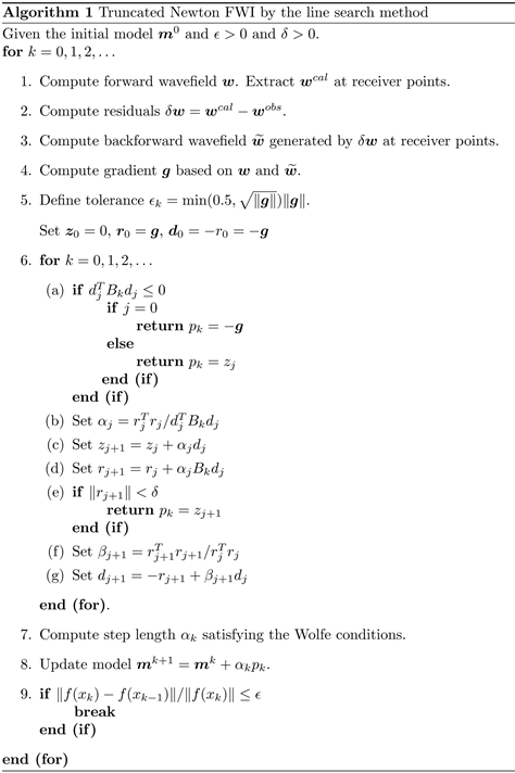
In this section, we present the algorithm of the truncated Newton method with the line search strategy and the algorithm of the Gauss-Newton method with the trust-region strategy.
Algorithm 1 is the FWI algorithm by using the truncated Newton method based on the line search method. There are two loops in Algorithm 1. The outer loop is the iteration of the line search strategy, and the inner loop is to compute the iterative direction
and the step length
. The core of the inner loop is Hessian-vector product
and so on. Algorithm 2 is the FWI algorithm by using the Gauss-Newton method based on the trust region method. In Algorithm 2,
is the Hessian approximation by the Gauss-Newton method. Comparing Algorithm 1 and Algorithm 2, we know the starting part of both algorithms is the same. The difference is in the rear part of the algorithm. In Algorithm 1, the line search strategy consists of the function of computing the step length and the iterative direction. On the contrary, in Algorithm 2, the trust region strategy combines the two steps together.

3. Numerical Computations
In this section, numerical computations are presented to illustrate the advantages of the trust region method. We also present the inversion results by the L-BFGS method for comparisons. We choose the L-BFGS method to make comparison as it is the most popular quasi-Newton method.
We consider FWI for the Marmousi model which is usually applied to test the ability of an imaging or inversion algorithm. The exact Marmousi model is shown in Figure 1. Figures 1(a)-(c) are the density, P-wave and S-wave velocities respectively. The model is 10 km in length along horizontal direction and 3.48 km
![]()
Figure 1. The exact Marmousi model. (a) Density; (b) P-wave velocity; (c) S-wave velocity.
in depth. It is grided by the 500 × 174 mesh with 20 m spatial steps in both
and
directions. We set 100 sources and 400 receivers in the data acquisition. The sources are located at 40 m in depth and the first source is set at
in the horizontal direction. The receivers are located at 460 m in depth with the first receiver is set at
in the horizontal direction. The source space is 40 m and the receiver space is 20 m. The source is the Ricker wavelet with the time function as
(3.1)
where
and
is the central frequency. The source is loaded on the
component. The recording time is 6 s with the time interval 2 ms.
For the elastic wave FWI, the density is more sensitive than the velocities. Some hierarchical inversion strategies developed by [13] and [14] can be applied. In our FWI computations, we don’t apply these strategies. We invert the three media parameters simultaneously. However, a multiscale technique by implementing the inversion from low frequency to high frequency is still used. Moreover, the data of the next high frequency band include the data of the previous low frequency band which guarantees the robustness of inversion. In our computations, four groups of frequencies are used to complete inversion step by step, i.e., 2 Hz, 5 Hz, 10 Hz and 20 Hz. For every stage, the stopping criterion is
(3.2)
where
is in fact the objective function computed by (2.8), and
is set 0.01 in our computation. This stopping criterion is based on the relative decrease of the misfit function.
The initial model for FWI is shown in Figure 2. Figures 2(a)-(c) are the initial density, P-wave and S-wave velocities respectively. They are generated by arithmetic average smoothing for the exact model along the depth direction only. In Figure 2, we can see there are no geological structures such as the faults in the initial model like those in the exact model.
The final inversion result by the Gauss-Newton method with the line search strategy is shown in Figure 3. The final inversion result by the Gauss-Newton method with the two dimensional subspace strategy is shown in Figure 4. The final inversion result by the truncated Newton method with the line search strategy is shown in Figure 5. We also complete the FWI by the L-BFGS. The results are similar and we omit the figures for saving space. We remark that the Hessian in the truncated Newton method is not positive and so the two dimensional subspace strategy can not be applied directly. Comparing Figures 3-5 with Figure 1, we can see that both the Gauss-Newton method and the truncated Newton method with the line search strategy can yield good imaging results. And the case of the Gauss-Newton method with the two dimensional subspace strategy is the same.
Figure 6 shows the profile comparison at the position
among the
![]()
Figure 2. The initial model for FWI. (a) Density; (b) P-wave velocity; (c) S-wave velocity.
![]()
Figure 3. The finial inversion result of Marmousi model by the Gauss-Newton method with the line search strategy. (a) Density; (b) P-wave velocity; (c) S-wave velocity.
![]()
Figure 4. The finial inversion result of Marmousi model by the Gauss-Newton method with the two dimensional subspace strategy. (a) Density; (b) P-wave velocity; (c) S-wave velocity.
![]()
Figure 5. The inversion result of Marmousi model by the truncated Newton method with the line search strategy. (a) Density; (b) P-wave velocity; (c) S-wave velocity.
![]()
Figure 6. The comparison of inversion results at
inverted by the L-BFGS method, the Gauss-Newton method and the truncated Newton method with the line search strategy. (a) Density; (b) P-wave velocity; (c) S-wave velocity.
inversion results by using the L-BFGS method, the Gauss-Newton method and the truncated Newton method with the line search strategy. In Figure 6, we can see both the inversion results of P-wave velocity and S-wave velocity obtained by the three methods are almost the same. However, the inversion results of density by the Gauss-Newton method and the truncated Newton method are obviously better than the L-BFGS method especially in deep positions.
In Table 1, we present the iteration number at every stage (i.e., 2 Hz, 5 Hz, 10 Hz and 20 Hz) for the L-BFGS method, the Gauss-Newton (GN) method and the truncated Newton (TN) method by the line search (LS) strategy or the two dimensional subspace (Sub) strategy. From Table 1, we can see that the Gauss-Newton method has obvious advantage over other methods from point of total iteration number.
In Table 2, we compare the computational efficiency for different methods. The total computational time and the time of each iteration are listed in Table 2. The total iteration number is also listed for convenience. As we can see, the Gauss-Newton method with the two dimensional subspace method costs least computational time for each iteration.
In Figure 7, we present a profile comparison of the inversion results at
by the Gauss-Newton method with the line search strategy and the trust region strategy. Figures 7(a)-(c) are the inversion results of density, P-wave velocity and S-wave velocity respectively. We can see that both strategies almost have the same inversion accuracy for P-wave velocity and S-wave
![]()
Table 1. The number of iterations at each stage for the L-BFGS method, the Gauss-Newton (GN) method and the truncated Newton (TN) method with the line search (LS) strategy or the two dimensional subspace (Sub) strategy.
![]()
Table 2. The total computation time and the time of each iteration for different inversion methods with the line search (LS) strategy or the two dimension subspace (Sub) strategy.
![]()
Figure 7. The comparison of inversion results for the Marmousi model at
inverted by using the Gauss-Newton method with the line search strategy and the trust region strategy. (a) Density; (b) P-wave velocity; (b) S-wave velocity.
velocity. For the density, we can see the trust region strategy with the two dimensional subspace strategy has better inversion accuracy than the line search strategy. In Table 3, we present
errors and relative
errors for the different methods. The relative error
is defined by
(3.3)
where
is the exact model and
is the inversion result. The relative
error for the truncated Newton method with the two dimensional subspace strategy is 7.28% and it is the least. This fact is consistent with the theory since the Newton method contains the full information of Hessian. For the Gauss-Newton method, we can see that the relative
error by the two dimensional subspace strategy is 7.38% whereas it is 7.49% for the line search strategy. It shows that the two dimensional subspace strategy is helpful to improve the inversion accuracy. Figure 8 shows the absolute
errors of inversion results versus iteration for the L-BFGS method, the Gauss-Newton method and the truncated Newton method.
![]()
Table 3. The
errors and relative
errors of final inversion results for different inversion methods with the line search (LS) strategy or the two dimension subspace (Sub) strategy.
![]()
Figure 8. The absolute
errors of inversion results versus iteration for the L-BFGS, the Gauss-Newton method and the truncated Newton method.
4. Conclusions
In FWI, the line search strategy is usually applied. In this paper, we have investigated the application of the trust-region strategy to elastic wave multi-parameter inversion. The theoretical methods and algorithms are described in detail. The trust-region subproblem is solved by the two-dimensional subspace method. Numerical computations for Marmousi model by the Gauss-Newton method and the truncated Newton method in the time domain are completed and compared.
We also have presented the corresponding inversion result by the L-BFGS method for comparison since it is the most popular quasi-Newton method. The comparisons demonstrate that both the Gauss-Newton method and the truncated Newton method are more accurate than the L-BFGS method. The trust region strategy is more efficient than the line search strategy. In the line search strategy, the information of Hessian and gradient is utilized for deciding the search direction whereas the search direction and the search step are determined together in the trust region strategy. In the trust region method, as long as the trust-region radius is well updated, the model updating can be performed for every iteration with the fixed trial step and there are no more extra computations of the forward problem. This is the theoretical reason why the trust-region strategy can save computational time. In the trust-region strategy, the two-dimensional subspace method requires that the Hessian matrix is positive and definite. Unfortunately, this condition is not always satisfied for the truncated Newton method. Future work will be the other measures to update the trust-region radius and the application of the trust-region method to other methods.
Acknowledgements
This work was supported by the National Natural Science Foundation of China under grant number 11471328. It is also supported by the Key Project National Natural Science Foundation under grant number 51739007. The computations in this paper are completed on the parallel cluster of State Key Laboratory of Scientific and Engineering Computing.
Appendix A. The Staggered-Grid Schemes for Solving (2.3)
Let
be the time step in the time direction and
the spatial step in
and
directions. The discrete indexes for
,
and
are denoted by
,
and
respectively. Then the difference schemes for
and
with the second order accuracy are
(A.1)
(A.2)
where
The difference schemes for strain
,
and
with the second order accuracy are the following
(A.3)
(A.4)
(A.5)
where
Appendix B. The Derivation for Gradient Formulae (2.16)-(2.18)
Note that
. (B.1)
Substituting (B.1) into (2.13), we have
(B.2)
which is just (2.16).
From the relation of strain and stress [19], we have
(B.3)
(B.4)
where
and
are the displacement in the
and
directions respectively. Adding (B.3) and (B.4) together, we have
(B.5)
that is
(B.6)
Similarly, for the backward wavefield
and
, we have
(B.7)
where
,
,
and
are the backward wavefield of the adjoint problem. Substituting (B.6) and (B.7) into (2.14), we get
(B.8)
which is just (2.17).
Since
(B.9)
we have
(B.10)
and
(B.11)
where
is the backward stress field corresponding to
. Multiplying (B.10) and (B.11), we obtain
(B.12)
Subtracting (B.3) and (B.4), we have
(B.13)
that is
(B.14)
Similarly, we have
(B.15)
Multiplying (B.14) and (B.15), we have
(B.16)
Multiplying (B.6) and (B.7), we have
(B.17)
Adding (B.16) and (B.17) together, we have
(B.18)
Substituting (B.12) and (B.18) into (2.15), we have
(B.19)
which is just (2.18).