The Triangular Hermite Finite Element Complementing the Bogner-Fox-Schmit Rectangle ()
1. Introduction
The finite elements with inter-elemental continuous differentiability are more complicated than those providing only continuity. Such two-dimensional elements are mostly developed for triangles: the Argyris triangle [1], the Bell reduced triangle [2], the family of Morgan-Scott triangles [3], the Hsieh-Clough-Tocher macrotriangle [4], the reduced Hsieh-Clough-Tocher macrotriangle [5], the family of Douglas-Dupont-Percell-Scott triangles [6], and the Powell-Sabin macrotriangles [7]. The Fraeijs de Veubeke-Sander quadrilateral [8] and its reduced version [9] are also composed of triangles. As for single, noncomposite rectangles, the Bogner-Fox-Schmit (BFS) element [10] is the most popular and simplest one in the family of elements discribed by Zhang [11]. All these elements are widely used in the conforming finite element method for the biharmonic equation and other equations of the fourth order (see for example [12-18] and references therein) along with mixed statements of problems and a nonconforming approach [12,14,17].
A direct application of the BFS-element is restricted to the case of a simple domain that is composed of rectangles or parallelograms whose sides are parallel to two different straight lines. This condition fails even in the case of a simple polygonal domain where the intersection of the boundary with rectangles results in triangular cells (cf. Figure 1). Of course, one can construct the special triangulation compatible with the boundary as some isoparametric image [19] of a domain composed of rectangles with sides parallel to the axes. This way requires solving some additional boundary value problems for the construction of such a mapping that is smooth over the whole domain.
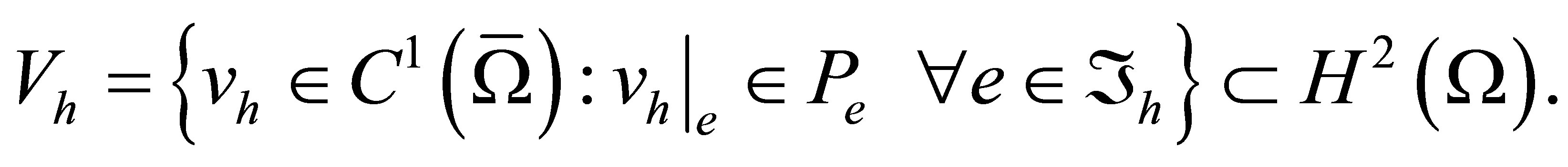
In this paper we suggest to use the BFS-elements in the direct way (without an isoparametric mapping) for a couple with the proposed triangular Hermite elements with 13 degrees of freedom. These triangular elements supplement BFS-elements in the following sense. They are used only near the boundary of a polygonal domain and provide inter-element continuous differentiability between finite elements of these two types. Thus, due to the joint use of these elements on a polygonal domain , the approximate solution of finite element method belongs to the class
  of functions which are continuously differentiable on the closure
  of the domain.
2. Triangulation of a Domain and the Bogner-Fox-Schmit Element
Let  be a convex polygon with a boundary
  Assume that we can construct a triangulation
  of
of  subdividing it into closed rectangular and triangular cells so that the most of them are rectangles and only a part of the cells adjacent to the boundary may be rectangular triangles. Besides, any two cells of
  may not have a common interior point and any two triangular cells may not have a common side. In addition, the union of all the cells coincides with
  A simple example of the triangulation is shown in Figure 1. We also assume that all sides of the rectangular cells and the catheti of the triangular cells are parallel to the axes.
Denote by  the maximal diameter of all meshes
 . On rectangular cells we use the Bogner-FoxSchmit element [1]. It is defined by the triple
where  is the rectangle with vertices
 and
and 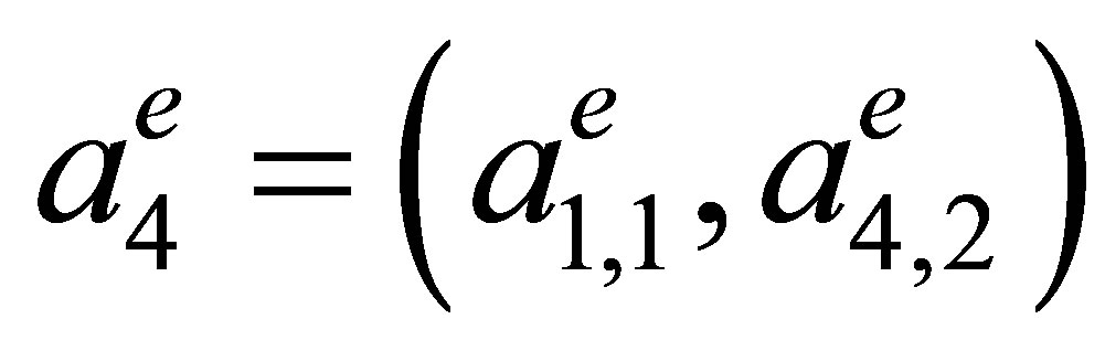
and with side lengths  and
and 
Besides,  is the space of bicubic polynomials on
  and
and  is the set of linear functionals (degrees of freedom or nodal parameters) of the form [12]
 (1)
(1)
The dimension of  (the number of the coefficients of a polynomial) is equal to 16 and coincides with the number of the degrees of freedom. For this element we have the Lagrange basis in
  that consists of the functions
 satisfying the condition
 (2)
(2)
where  is the Kronecker delta. These functions can be written in the explicit form with the help of the one-dimensional splines

Indeed, the direct calculations show that the basis has the form
 ,
,

3. The “Reference” Triangular Hermite Element
First we construct the “reference” triangular element  with the specified properties. We consider the right triangle
  which has 4 nodes
  with the coordinates (0, 0), (1, 0), (0.5, 0.5), and (0, 1), respectively (Figure 2).
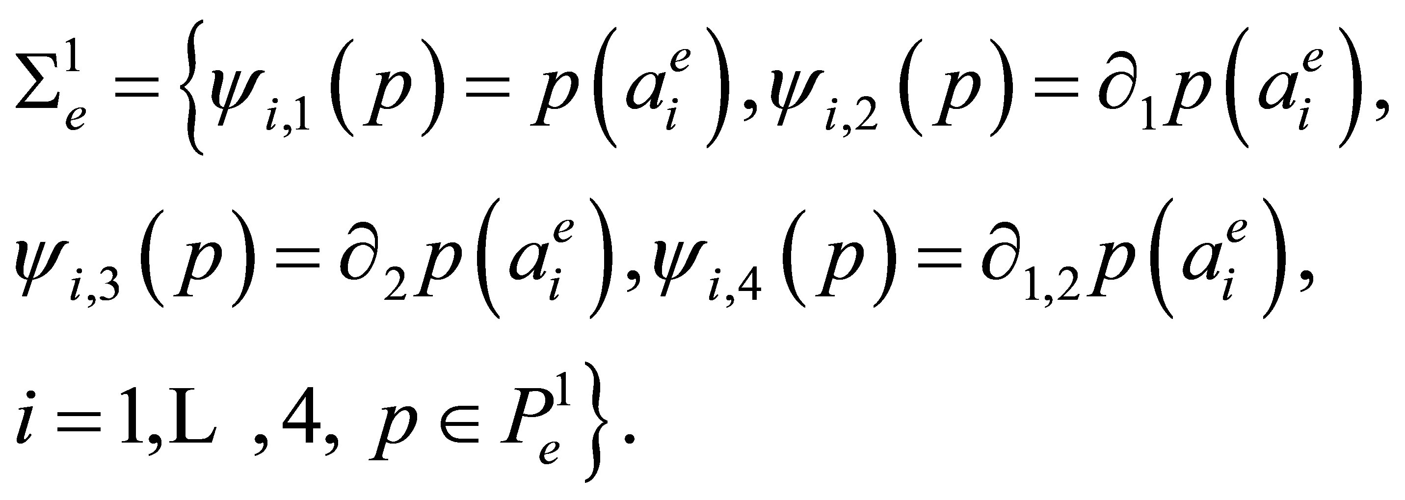
We define the space  of functions and the set
  of degrees of freedom as follows:
 (3)
(3)
Figure 2. The “reference” triangular element.
Observe that at each of the nodes , and
, and  there are 4 degrees of freedom and at the node
  there is only one degree. Besides, the degrees of freedom for the nodes
 , and
, and  coincide with those for the nodes of the BFS-element (1).
Lemma 1. The triple  is a finite element.
Proof. The dimension of the space  coincides with the number of elements of the set
  Hence, to prove unisolvence of the couple
 , it is sufficient to construct the Lagrange basis {
 where
where  for i = 1, 2, 4 and j = 1 for
  } on
} on  satisfying the condition [12]
 (4)
(4)
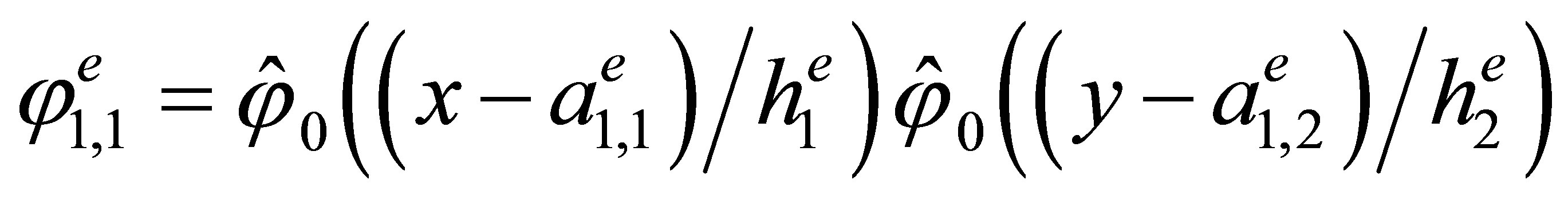
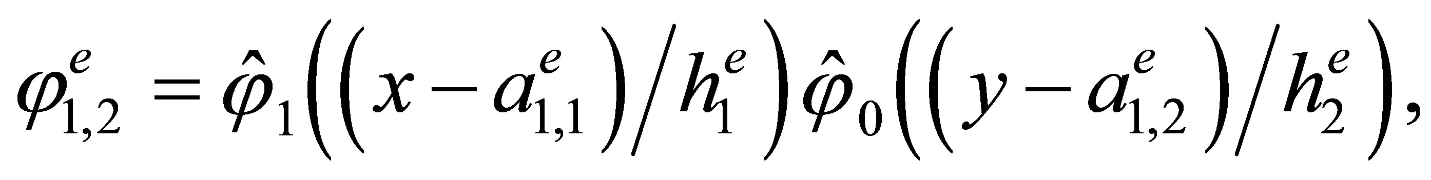
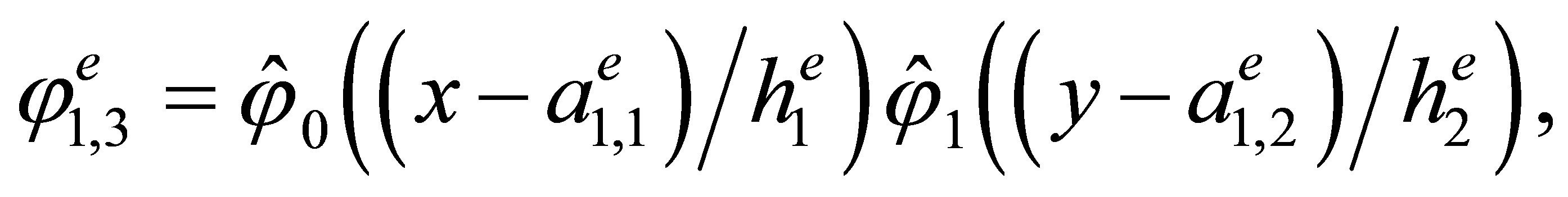
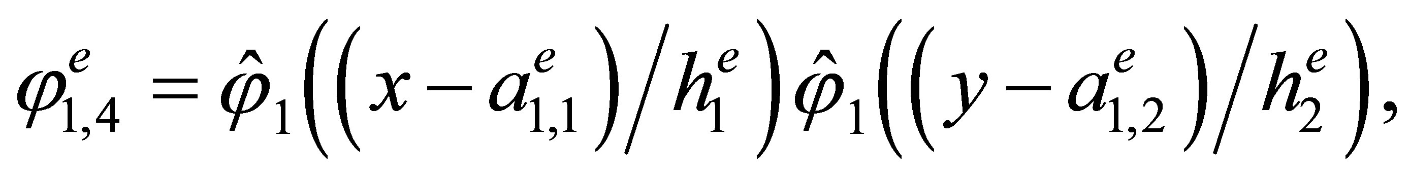
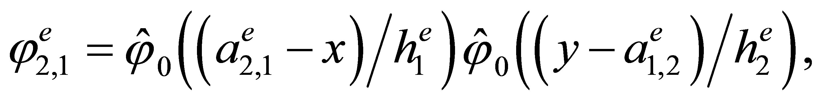
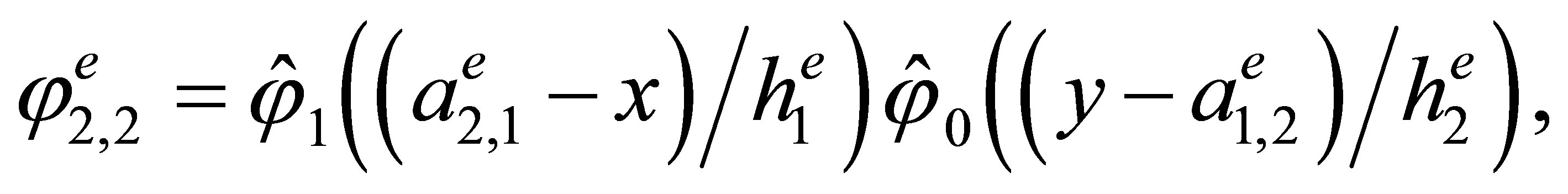
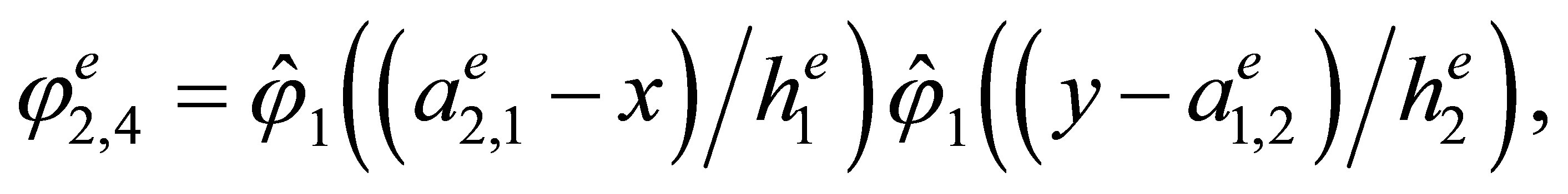
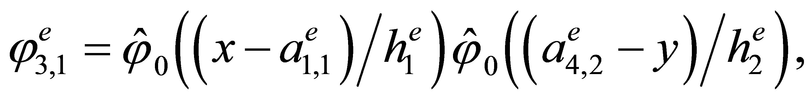
The direct calculations show that the Lagrange basis has the following form:
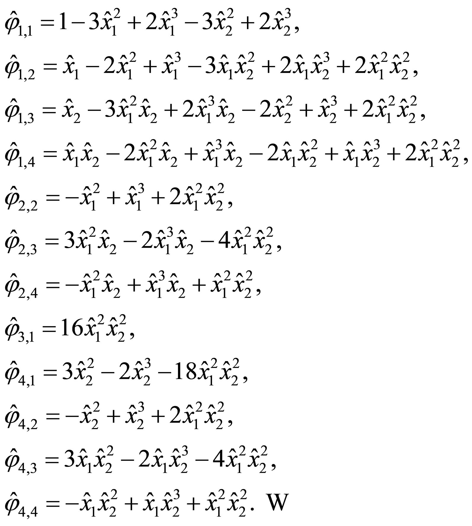 (5)
(5)
Let  be an arbitrary function. Along the side
  it is a polynomial of degree 3 in
  Together with the derivative
  it is uniquely determined by the values
 , and
, and  of nodal parameters. In addition, the derivative
  along
along  is a polynomial of degree 3 in
  as well and is uniquely determined by the values
 and
and  of nodal parameters. On the side
similar statements are valid within the replacement of  by
by 
Thus, on the sides  and
and  the values of a function of
  and its first-order partial derivatives are uniquely determined by the values of nodal parameters of
  at the nodes on the corresponding side.
On the side  a similar property does not hold. Generally speaking, the element
  is not of the class
 . This follows from the fact that the firstorder partial derivatives of the basis functions related to the node
  do not vanish on the side
 . However, further we assume that the side of any triangular element of
  being the image of the hypotenuse
  is a part of the boundary and can not be a common side of two meshes. Hence, this feature has no influence on interelemental continuity inside the domain.
To check the interpolation properties, we use the usual notations for Sobolev spaces. Here  is the Hilbert space of functions, Lebesgue measurable on
  equipped with the inner product
and the finite norm
For integer nonnegative 
 is the Hilbert space of functions
  whose weak derivatives up to order
  inclusive belong to
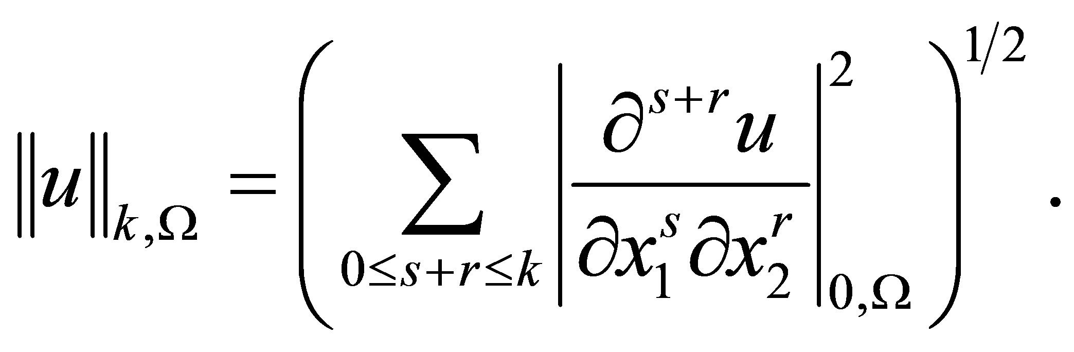
 . The norm in this space is defined by the formula
We also use the seminorm
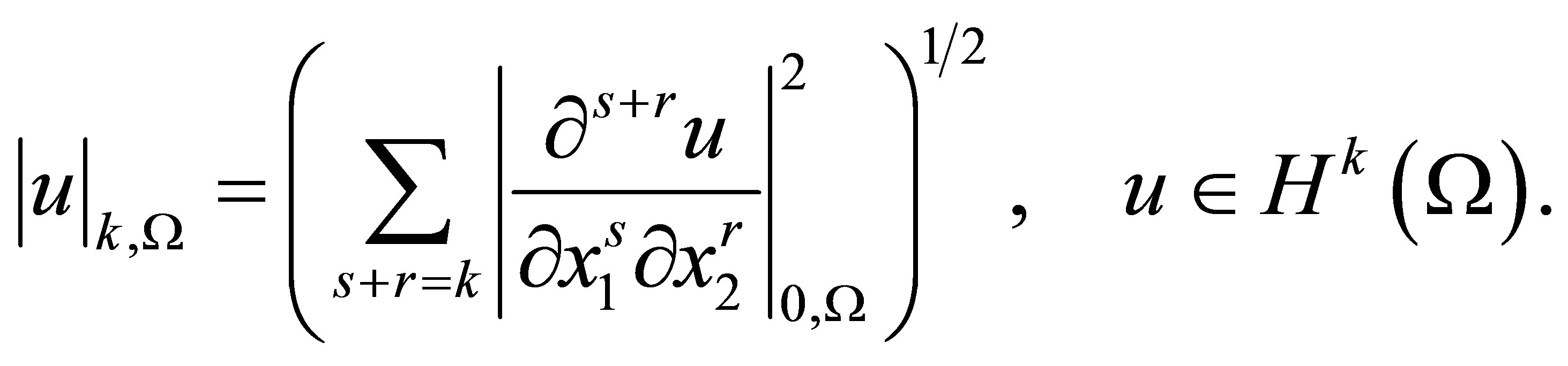
Let  be an arbitrary function of
  By a Sobolev embedding theorem,
  is continuously embedded into
  [20], hence,
 . Thus, we can construct its interpolant
  Denote by
  the number of degrees of freedom related to a node
  We have
Theorem 1. Let  Then for any integer
  we have the estimate
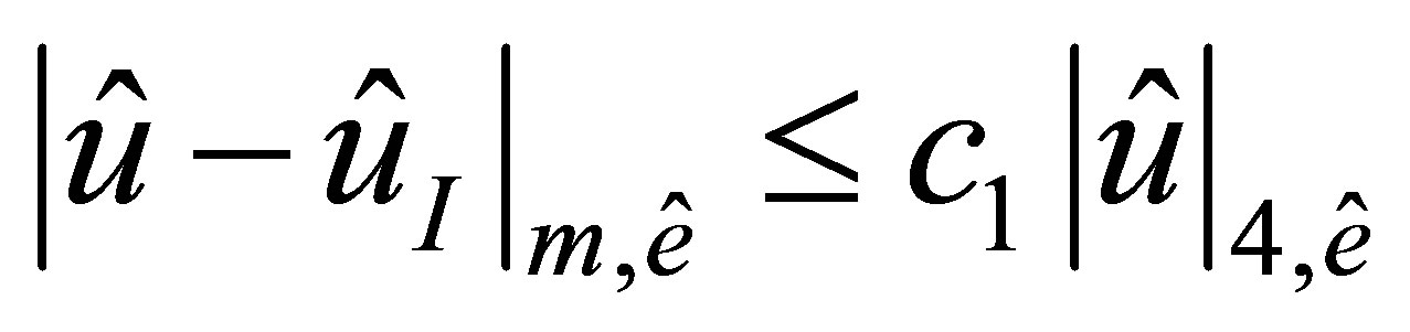 (6)
(6)
with constant  independent of
  (and
(and ).
).
Proof. The maximal order of partial derivatives equals 2 in the definition of the set  As mentioned above, the space
  is embedded into
  Besides, from (3) it follows that
  where
where  is the space of polynomials of degree no more than 3.
Thus, all the hypotheses of the Theorem 3.1.5 in [12] are fulfilled, which implies the estimate (6). ,
4. Combination of Rectangular and Triangular Elements
Let  be an arbitrary triangular element (Figure 3) with vertices
 and side lengths
 The affine mapping
 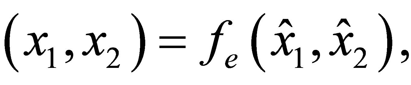 that maps the «reference» element
  into е, has the form
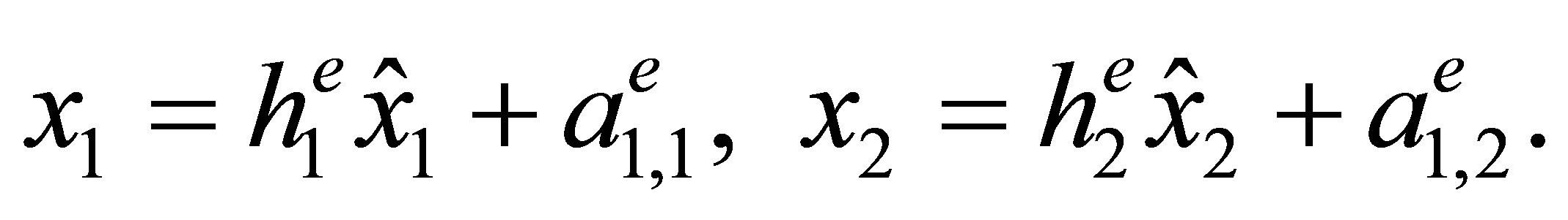 (7)
(7)
We specify the space  of functions and the set
  of degrees of freedom as follows:
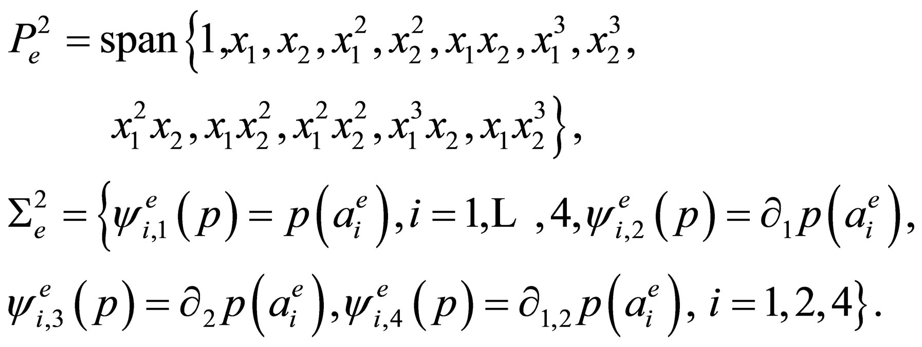 (8)
(8)
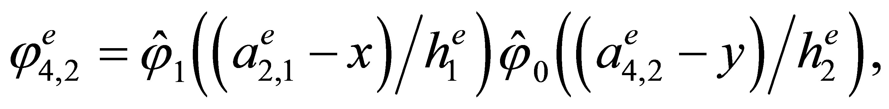
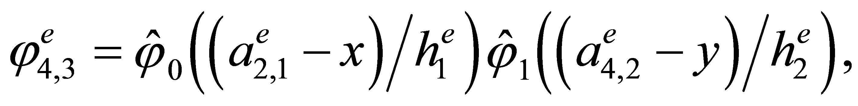
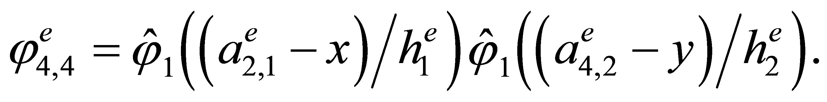
The Lagrange basis in  consists of the functions
 , where
  for i = 1,2,4 and j = 1 for i = 3 being the images of the basis (5) under the mapping (7) and satisfying the condition
 (9)
(9)
Thus, the triple  is a finite element that is affinely equivalent to the «reference» element
  [12].
[12].
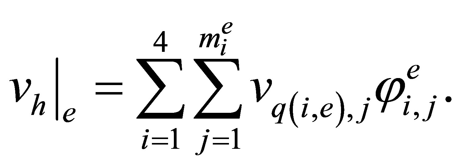
Now denote the set of all nodes of the elements  by
by  and number them from 1 to
  With each node
  we associate the number
  equal
equal
to the number of degrees of freedom related to this node. Observe that  is occurred when the node
  is the midpoint of the side of a triangular element being a part of the boundary
  and
and  for all remaining nodes of
This is the global numbering of nodes. We also introduce the local numbering. The couple  is assumed to be a local number of the node
  of an element
 . To any local number
  there corresponds one and only one global number
  hence, we can introduce the function
  so that
  In addition, for an element
  we denote the local analogue of the parameter
  by
by , i.e.,
  for
for 
At each node ,
,  , we specify
  numbers
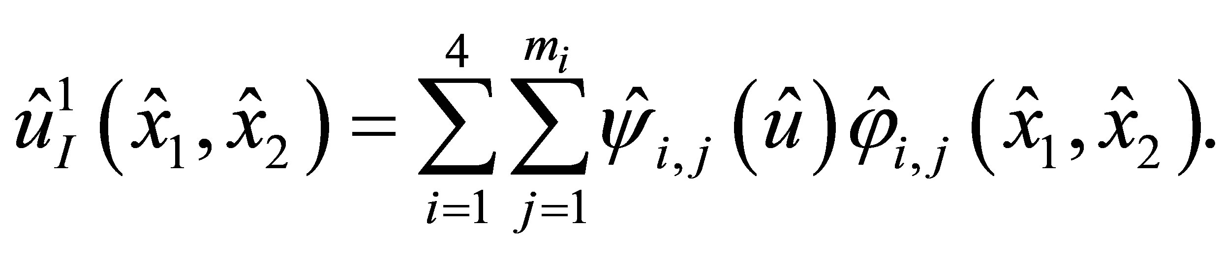
  Construct the function
  defined on
  such that
 (10)
(10)
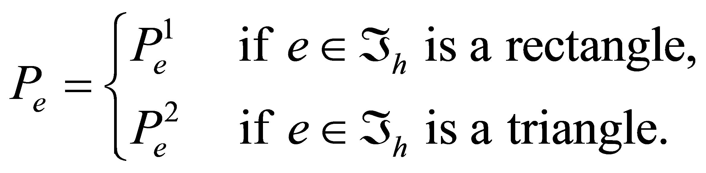
By the construction, the function  is uniquely defined on each
 . Put
. Put
Then 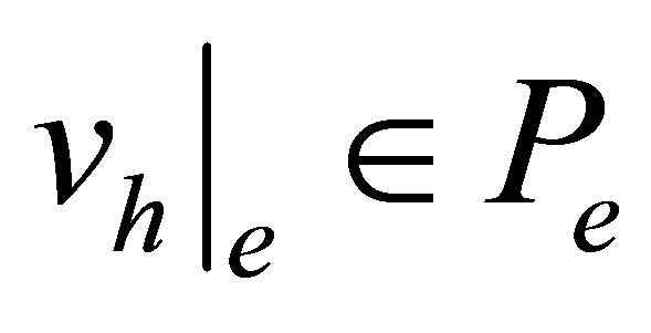 for any
Lemma 2. The function  defined by the relation (10) belongs to
Proof. The BFS-rectangles are elements of the class  i.e., the function
  and its first-order derivatives are continuous on the sides common for two elements of this type [10].
Now let  be an arbitrary triangular cell and
  be a rectangular cell that has a common side
  with
with  (Figure 4). Because of construction, the values of the nodal parameters of the functions
  and
and  on
on  are equal. In addition, the traces of these functions and their first-order derivatives with respect to
  on
on  are polynomials of degree 3 in
  and are uniquely defined by the sets of nodal parameters related to the side
 . Hence, the functions
  and
and  coincide on
 along with their first-order derivatives. ,
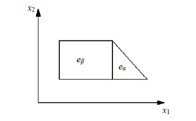
Figure 4. Two neighbouring elements of different types.
Corollary 1.  [12,21]. Thus, we can define the finite element space as follows:
Let . Define its interpolant
  in the following way:
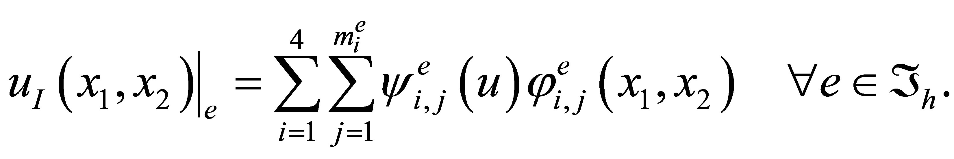 (11)
(11)
With the help of the Theorem 1, the following estimate can be proved in the usual way (see, for instance, [12,14]).
Theorem 2. Assume that  And let
  be its interpolant defined by (11). Then
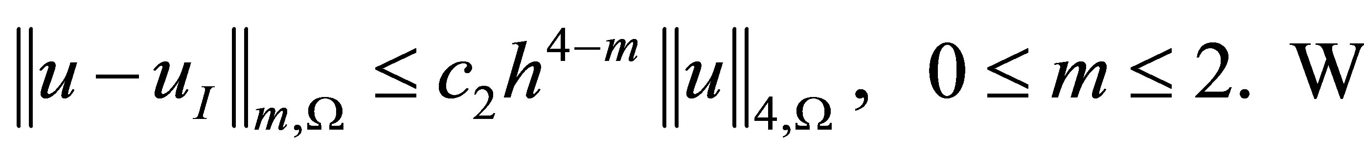
Here and later constants  are independent of
  and
and 
5. Numerical Example
We illustrate properties of the proposed finite elements by the following example. Let  be a right triangle with unit catheti (see Figure 5) and a boundary
  Consider the problem
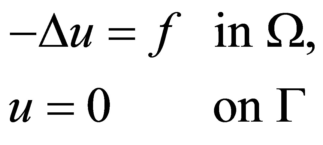
with the right-hand side

It has the exact solution
Subdivide the domain  into elementary squares (with triangles adjacent to the hupotenuse) by drawing two families of parallel straight lines
  and
and  with mesh size
To compare accuracy with decreasing mesh size, we construct a system of linear algebraic equations of the finite element method with the BFS-elements on the elementary squares and the proposed elements on the
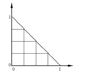
Figure 5. Domain Ω with initial triangulation.
triangles for  Since the exact solution is known, the difference
  between exact and approximate solutions can be expressed in the explicit form. As a result, we have the following accuracy.
Theoretically, in the finite element method we have the estimate [12,14]
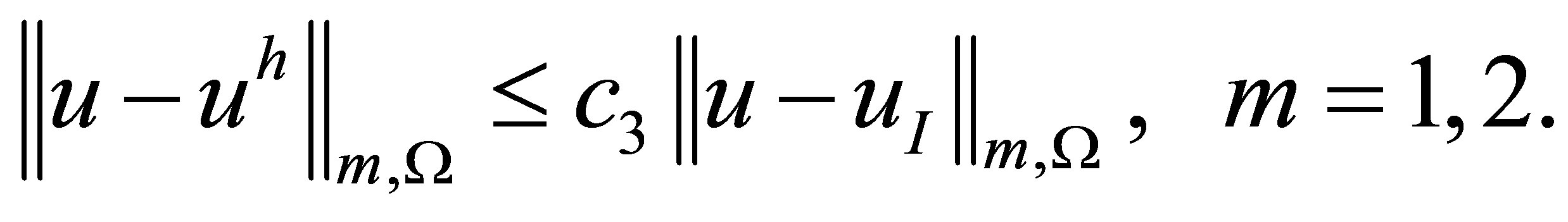
Combining it with the estimate in Theorem 2, we arrive at the following error estimate for an approximate solution:
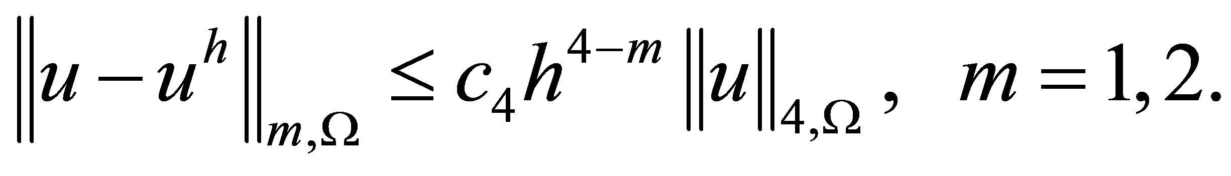 (12)
(12)
Comparing the last two results in Table 1, observe that they are close to the asymptotic values 4 and 3, respectively.
6. Summary and Further Implementations
Thus, the use of the proposed triangular finite elements only near a boundary extends the field of application of the BFS-elements at least for second order equations. In its turn, an approximate solution is of the class  enabling one to calculate a residual directly and considerably simplifies a posteriori accuracy estimates for an approximate solution.
In principle, to achieve the same order accuracy, instead of the BFS-elements, one can use the Lagrange bicubic elements on rectangles and the Lagrange elements of degree three on triangles. But in this case a general advantage of Hermite finite elements in comparison with Lagrange ones makes itself evident in the number of unknowns of a discrete system. In particular, Table 2 shows the number of degrees of freedom for an approximate solution which is equal to the number of unknowns and the number of equations in a discrete system of linear algebraic equations for the example from the above section.
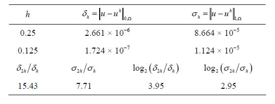
Table 1. Accuracy of an approximate solution.
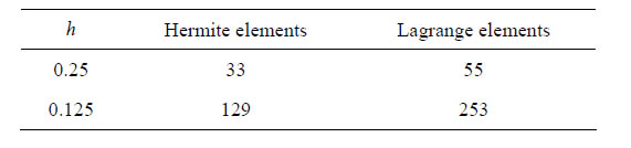
Table 2. The numbers of degrees of freedom for an approximate solution.
Observing a considerable gain in the number of unknowns, with the further refinement of triangulation, the number of unknowns (and equations) asymptotically tends to the ratio of 4:9 in favour of Hermite elements.
Now we notice an apparent inconvenience and show a way to overcome it that is also useful for nonconforming grid refinement. The triangulation shown in Figure 1 is constructed by adjusting cells of a rectangular grid in the  - and
- and  -directions. It imposes restrictions on the ratio of steps for a rectangular grid inside a domain. We show that the proposed triangular elements are sufficient to construct a conforming interpolant, generally speaking, on an “uncoordinated” grid without restriction on the ratio between steps.
Considering a typical case shown in Figure 6, the node  is a so-called “hanging” node. At the algorithmic level, the challenge is solved as follows. For the degrees of freedom at the node b, instead of the corresponding variational equations for an approximate solution
  we write 4 linear algebraic equalities which express the quantities
  and
and  in terms of 16 degrees of freedom of the neighbouring rectangle
  This trick ensures interelemental continuous differentiability of an interpolant between
  and
and  Thus in this case one again may implement proposed pair of elements in the frame of the conforming finite element method with estimate (12).