1. Introduction
The special matrix functions appear in statistics, lie group theory and number theory [1-4] and the matrix polynomials have become more important and some results in the theory of classical orthogonal polynomials have been extended to orthogonal matrix polynomials see for instance [5-9].
If  is the complex plane cut along the negative, real axis and log
 denotes the principal logarithm of z (Saks, S. and A. Zygmund, [10]), then
  represents
  if A is a matrix in
  the set of all the eigenvalues of is denoted by the set of all the eigenvalues of A is denoted by
 . If
. If  and
and  are holomorphic functions of the complex variable z, which are defined in an open set
  of the complex plane, and A is a matrix in
  such that
 . Then from the properties of the matrix functional calculus, (Dunford N. and J. Schwartz J. [11]), it follows that
 . If A is a matrix with
  , then
  denotes the a image by
  of the matrix functional calculus acting on the matrix A. we say that A is a positive stable matrix if
  for all
 .
.
For any matrix P in  we will exploit the following relation due to [12]
 (1)
(1)
Khammash [12], define the Gegenbauer matrix polynomials of two variables by
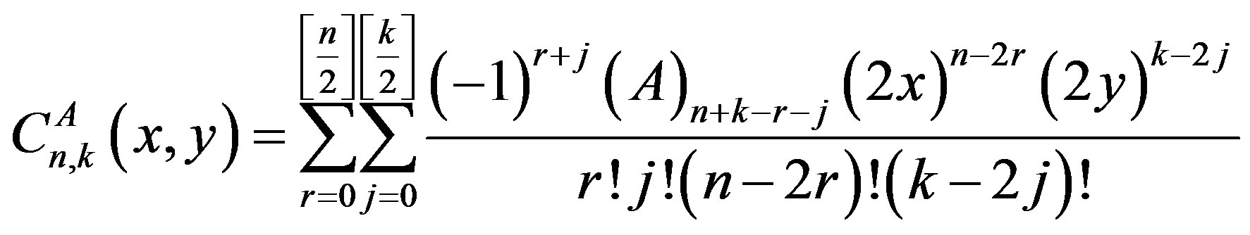 (2)
(2)
From which it follows that  is a matrix polynomial in two variables x and y of degree precisely n in x and k in y.
Also we recall that if  are matrix in
  for
for  and
and  that it follows that (Defez and Jódar [14])
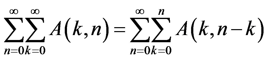 (3)
(3)
 (4)
(4)
and, for m is a positive integer such that , then
 (5)
(5)
 (6)
(6)
We define Humbert matrix polynomials of two variables and discuss its special cases. Some hypergeometric matrix representations of the Humbert matrix polynomials of two variables, the double generating matrix functions and expansions of the Humbert matrix polynomials of two variables in series of Hermite polynomials are given. Some particular cases are also discussed.
2. Definition of Humbert Matrix Polynomials of Two Variables
Let A be a positive stable matrix in  for a positive integer m, we define Humbert matrix polynomials by
 (7)
(7)
Now (7) it can be written in the form

and by (3) and (6) respectively, one gets
 (8)
(8)
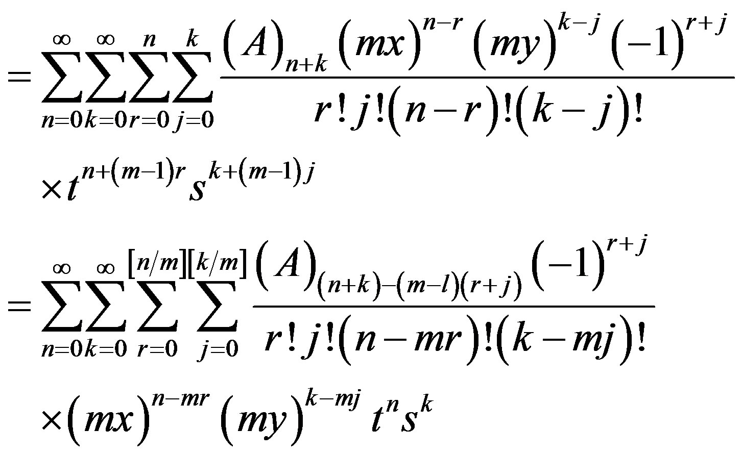
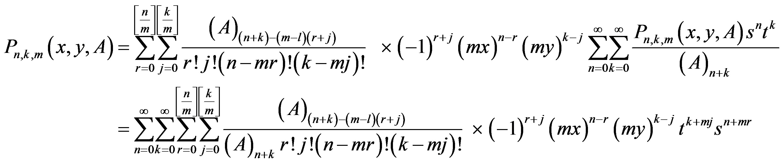
By equating the coefficients of  in (7) and (8), we obtain an explicit representation of the Humbert matrix polynomials of two variables. In the form
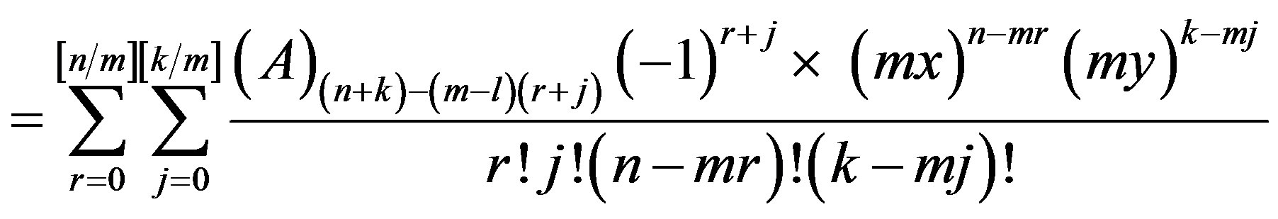 (9)
(9)
from which it follows that  is a matrix polynomial in two variables x and y of degree precisely n in x and k in y. In (9) setting m = 2, we get the Gegenbauer matrix polynomials of two variables [13] as particular case of the Humbert matrix polynomials of two variables.
3. Hypergeometric Matrix Representation for 
We study here the representation of the hypergeometric matrix representation for the Humbert matrix polynomials of two variables. There are some facts and notations used throughout the development in Sections 3 - 5, which are listed here.
Fact 1. [15] The reciprocal scalar Gamma Function , is an entire functions of the complex variable z. Thus, for
 , the Riesz-Dunford functional calculus [11] shows that
  is well defined and is indeed, the inverse of
 , Hence: if
  is such that
  is invertible for every integer
 . Then
 .
.
Fact 2. [12] If A, B and C are members of  for which
  is invertible for every integer
 . The hypergeometric matrix function
  is defined by

it converges for .
.
Notation 1. [16] For , the matrix version of the pochhammer symbol (the shifted factorial) is
 (10)
(10)
with .
.
Note that , where j is a positive integer, then
  when ever
 . Also, the product in (10) is commutative, and then it is easy to see that

and

where m is a positive integer.
Notation 2. [17]


Now, in view of Notation 2, the explicit representation (9) for , becomes

Thus we get the following hypergeometric representation of Humbert matrix polynomials of two variables.
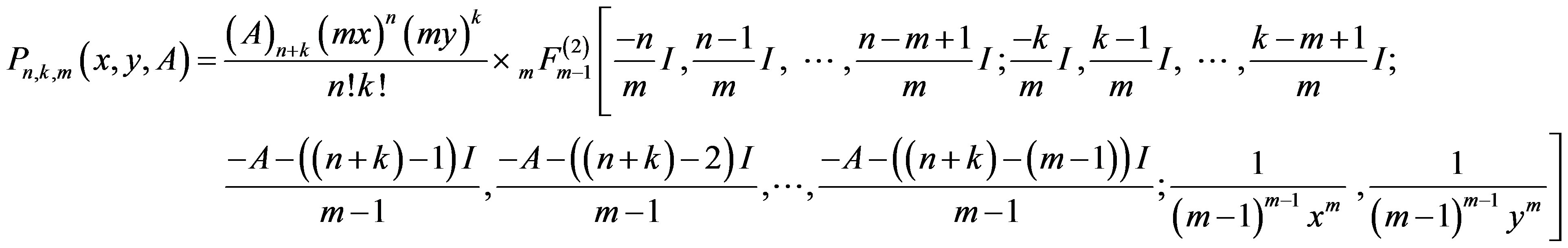 (11)
(11)
For m = 2 (11), we gives hypergeometric representation of Gegenbauer matrix polynomials of two variables [13].
The above facts and notations will be used throughout the next two sections.
4. Additional Double Generating Matrix Functions
Now, since
 (12)
(12)
By using (5), one gets
 (13)
(13)
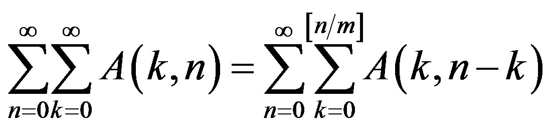
By using Notation 1, the following generating matrix functions for Humbert matrix polynomials of two variables follows

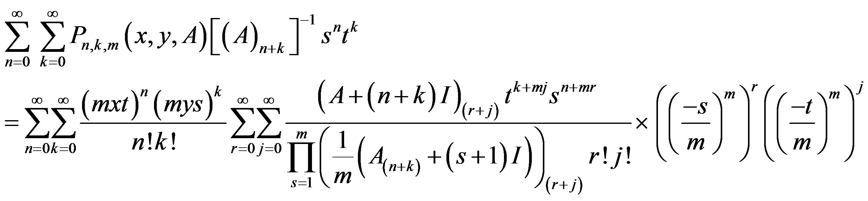
have thus discovered the family of double generating function of the Humbert polynomials of two variables
 (14)
(14)
If B is a positive stable matrix in , then let us now return to (12) and consider the double sum.

Then in similar manner, we get
 (15)
(15)
5. Expansions of  in Series of Hermite
Now, we derive expansions of  in series of Hermite
  According to [18], the expansion of
  in a series of Hermite matrix polynomials was given in the form:
 (16)
(16)
which with the aid of (5) and (9), one gets

From (16), we get

Now replacing  by
by  and equating the coefficients of
 , we get
 (17)
(17)