Review of Methods to Calculate Congestion Cost Allocation in Deregulated Electricity Market ()
1. Introduction
Since 1989, many countries followed the trend to unbundle their vertically integrated power utilities into several components in order to bring competition to the energy supply industry [1]. However, transmission congestion has added complication to the operation of the system. With the deregulation process, congestion management becomes more complex since transmission network access has to be open to all market participants and each participant should take responsibility for their congestion contribution [2]. Congestion could cause cheaper power not being delivered to the most desired load and that the congestion relief cost increases [3]. It is a challenge for the system operator to draw up a set of rules which must be robust, fair and transparent to the market and maintain the efficiency and reliability of the network [4]. Congestion cost allocation is based on two pricing schemes: uniform marginal price and locational marginal price [3]. The major difference between them is that uniform marginal price allocates cost uniformly to all loads without considering their locations and power flow contribution while locational marginal price does [5]. This paper reviewed above two pricing schemes with their mechanisms, pricing calculation and pros and cons. Then an IEEE-14-bus system is used as a test system simulated by the software Matpower to test the two methods on congestion cost allocation.
2. Uniform Marginal Price
2.1. Mechanism
The old England & Wales Pool was one of the pioneers for electricity industry deregulation in the world [2]. Uniform Marginal Price was implemented in this market as pricing scheme and congestion management method. Here the National Grid Company has two roles: transmission asset owner (TO) and Independent System Operator (ISO) [5] [6]. The ISO adopts the principle referred to as “re-dispatch first, compensate later” to manage transmission congestion which means it is a two stages operations [3]. In unconstrained dispatch stage, generation companies send generation bidding quantity and price of the following day to the ISO who already forecasted the power demand for each half hour period [1]. Then the ISO starts to accept bids from the cheapest price to higher price until the forecasted demand is satisfied. Then, the ISO sorts out a bid list which contains the generation companies who have been chosen to generate electricity. Those generation companies are called “in merit” generation companies and those who have not been accepted are called “out of merit” generation companies [2]. If there is no congestion violation, the unconstraint dispatch will be executed [5]. When transmission congestion occurs, it comes to the security-constrained stage and the ISO will re-dispatch the generation list, at the meantime ensuring the re-dispatch cost is the minimum. An inequality constraint will be added and the security re-dispatched is decided by the new algorithm. The congestion relief cost is the generation cost in security-constrained dispatch minus the generation cost in unconstrained dispatch. The congestion cost is allocated in equal proportional to each load while generators are not charged for transmission congestion [7].
2.2. Pricing Calculation
Congestion management is implemented through power energy prices and transmission usage charges [8]. In unconstrained dispatch, bid price of the last dispatched generator becomes the system marginal price (SMP) [2]. If there is no congestion violation, the ISO will execute the unconstrained dispatch and market participants will be paid and charged at the SMP. Once transmission congestion occurs, the ISO will implement re-dispatch and set a group of prices for generators and loads as follows [2]:
 (1)
(1)
 (2)
(2)
where:
PSP: Pool Selling Price, actual price charged for load
PPP: Pool Purchase Price, actual price paid to the generator
SMP: System Marginal Price
LOLP: Loss of Load Probability
VOLL: Estimated amount customers are willing to pay to avoid supply interruption
Uplift: The cost of power losses, ancillary service and congestion
LOLP is the probability that electricity power capacity is unable to support the actual demand [2]. After security-constrained dispatch, the ISO pays generators at PPP and charges loads at PSP. Neglecting power losses and ancillary service, the Uplift can be regarded as the cost of congestion relief and expressed as follows [2]:
 (3)
(3)
Congestion cost will be assigned to all loads and congestion cost assigned to load i as follows [5]:
 (4)
(4)
2.3. Pros and Cons
Uniform marginal price is a good innovation scheme to manage congestion after industry deregulation. Electricity prices barely reflect the congestion cost since the ISO ignores loads’ locations and power flow contributions. Generators are not charged for congestion so that correct signals are unable to pass to new market participant and transmission investment [7].
3. Locational Marginal Price
3.1. Mechanism
Locational Marginal Price (LMP) is the primary pricing scheme in the US electricity markets for congestion cost allocation. The definition of the LMP is the minimum marginal cost of the next increment of 1 megawatt hour power at a specific bus [9]. If there are no transmission congestion and losses, the LMP of each node will be the same. However, in reality, transmission congestion and losses will no doubt exist. When congestion happens, LMPs of different nodes become distinct due to variability of supply cost and available transmission capacity [10]. At a node, Generators are paid at their bid prices and loads are charged based on the LMP which is determined by the SO [5]. There is a possible trend that LMP will become the dominate congestion management since it has been adopted by many electricity markets in the US [11]. Take the PJM as an example, the LMP is utilized to calculate charges and payments in power delivery including spot market price and congestion cost [12]. There are two major markets in the PJM: a day-ahead market and a real-time balancing market. Both market prices calculation are based on the concept of the LMP [13]. LMP calculation is based on an optimization problem that maximizes the total social welfare function with balance equality which is equivalent to a minimization of an economic objective function subject to equality and inequality constraints of transmission network operation [10]. The SO uses optimal power flow (OPF) to calculate dispatch of each generator [14]. OPF model has two types: DCOPF and ACOPF. With non-linear equations, ACOPF demands a very long time to simulate large scale power system data. Compared with ACOPF, DCOPF is much simpler and a more convenient approach since it is linear and only considering active power flow whilst neglecting voltage, reactive power and transmission loss. As a result, DCOPF is often used for generator dispatch and LMP calculation [15].
3.2. Pricing Calculation
It is known that the sum of all power injected into all nodes is equal to sum of all power withdrawn from all nodes plus transmission losses which can be written as [2]:
 (5)
(5)
where:
 : Transmission losses in the power system
 : Sum real power generated from node i
 : Sum real power demand at node i
Based on the Equation (5), the the corresponding Lagrangian equation can be defined as follows [10]:
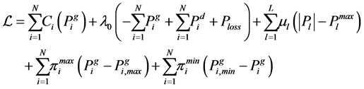 (6)
(6)
where:
 : Lagrangian multiplier of the whole system’s power balance constraint
N: Total number of nodes
L: Total number of transmission lines
 : Lagrangian multiplier of transmission line constraint
 : Lagrangian multiplier of maximum generation capacity of generator i
 : Lagrangian multiplier of minimum generation capacity of generator i
Based on the Equation (6), equation of LMP of node i can be obtained as follows [2]:
 (7)
(7)
where:
 : Sensitivity factor for real power at node i with line l constraint
From Equation (7), the LMP of a node i can be divided into three components as follows [11]:
 (8)
(8)
where:
 : System marginal cost of node i
 : Cost of transmission congestion of node i
![]() : Cost of transmission losses of node i
: Cost of transmission losses of node i
Combine Equation (7) and Equation (8), each component is shown as follows [11]:
![]() (9)
(9)
![]() (10)
(10)
![]() (11)
(11)
3.3. Pros and Cons
By utilizing LMP approach, economic signals are indicated and can be reflected to market participants. The influence of transmission congestion and losses will be reflected in the LMP variation of nodes so that electricity market is transparent. For longer-term view, LMP gives incentives for generation and transmission investments. Nevertheless, LMP cannot be regarded as a perfect approach. Because generation bids submitted to the SO is bid-based rather than cost-base, generator companies still have chance to act gaming behaviors [16]. Under transmission congestion circumstances, even though LMP can be effective, congestion revenue collecting from the SO will cause inefficiency for economic operation of the electricity market [14]. Power system networks are always huge so the designing work of LMP is significant complex and required large degree of coordination [2].
4. Case Study
A modified IEEE-14-bus system has been built by the software package Matpower as shown in Figure 1.
![]()
Figure 1. The diagram of the modified IEEE-14 bus model.
This model is used to calculate congestion cost allocation by Uniform Marginal Price and Locational Marginal Price. Before the test, some parameters should be set as follows in Table 1.
From Table 1, bid prices, maximum and minimum MW outputs of five generators and MW of each load are set. Branches parameters should also be set. In order to simulate congestion, branch between bus 1 and bus 2 has to be set as 60 MW. Using Matpower to simulate DCOPF, data of unconstrained dispatch and security-constrained dispatch is obtained as follows in Table 2 and Table 3.
Simulate Uniform Marginal Price method to calculate congestion cost allocation and the results are shown as follows in Table 4.
Using Matpower, the locational marginal prices of each load in unconstrained dispatch and security-constrained dispatch are obtained respectively as follows in Table 5.
![]()
Table 2. Generation cost of unconstrained dispatch and security-constrained dispatch.
![]()
Table 3. Branch flows of unconstrained dispatch and security-constrained dispatch.
![]()
Table 4. Allocated congestion cost (uniform marginal price).
Simulate Locational Marginal Price method to calculate congestion cost allocation and the results are obtained as follows in Table 6.
Pick up the fourth column of Table 4 and fifth column of Table 6, a comparison in congestion cost allocation on each load between two methods is shown in Figure 2; Pick up the third column of Table IV and the sixth column of Table VI, a comparison in congestion cost allocation per MW between two methods is also shown in Figure 2.
![]()
![]()
Figure 2. Comparison in congestion cost allocation and congestion cost allocation per MW.
![]()
Table 5. Allocated congestion cost (LMPs).
![]()
Table 6. Allocated congestion cost (locational marginal price)
5. Conclusion
From Figure 2, it is indicated that locational marginal pricing considers load’s location and power flow contribution so that the allocated congestion cost for L2 is larger than other loads since the transmission congestion occurred on branch 1-2. It is observed that congestion cost allocation in uniform marginal pricing is based on one non-dis- criminate price. It does not reflect load’s contribution to transmission congestion which means every load in the market shares the congestion cost uniformly. Locational marginal pricing provided economic signals to tell market participants where the congestion occurred. The participant, who contributes the congestion more, is required to pay for the congestion relief at a higher price.