A Probabilistic Approach for Studying the Reliability of Cementless Hip Prostheses in the Presence of Mechanical Uncertainties ()
Keywords:Probabilistic Analysis; Cementless Hip Prosthesis; Bone-Implant Interface; Primary Stability
1. Introduction
The amount of relative micro-movement between bone and implant plays a crucial role in the success of Total Hip Replacement (THR) [1]. Ideally, to promote the Primary Stability of the prosthesis, the amount of relative micro-movement between bone and implant induced early after the operation, before any biological process takes place, must remain lower than a prescribed threshold. If not, the lack of Primary Stability may lead to the aseptic loosening of the implant [1]. The primary stability of a cementless hip stem is not only affected by the implant design, but also by biomechanical properties, among which the coefficient of friction at the bone-implant interface or the elastic properties of the cancellous bone are known to play a crucial role. The natural variability of these parameters has to be taken into account to predict the Primary Stability of the THR. This is practically unfeasible experimentally, due to the great number of tests which would have to be carried out. The combination of numerical models and probabilistic methods offers a promising alternative.
Probabilistic methods enable the estimation of the effects of parameter variability in the resulting statistical variation of the system response to be determined. Each parameter is generally represented as a random variable, and the propagation of their randomness into the system response is predicted. By understanding the distribution of performance, evaluations of quality and risk assessment can be performed. Recent studies have proposed probabilistic approaches to assessing the structural integrity of orthopaedic implants [2-8]. Previously, Browne et al. [9] applied reliability theory to aid in fracture mechanics-based life prediction procedures for a tibial tray component represented as a cantilever beam subjected to constant amplitude loading. Dar et al. [10] demonstrated how Taguchi and probabilistic methods could complement each other to account for uncertainties when predicting stresses with finite element analysis, in a study of a fixation plate represented as a cantilever beam. The femoral stem component of a total hip replacement has been the subject of several probabilistic structural integrity studies [11]. Bah and Browne [12] used an idealized cylindrical finite element model to represent an implanted cemented hip stem in order to assess the most likely failure mode and to identify which parameters had the largest contribution, where geometry, material properties and loading were considered as random variables. The latest studies concerning the application of probabilistic approaches to cementless hip prostheses have focused on the effect of femur characteristics and implant design geometry [13] or implant positioning on Primary Stability [14].
This paper presents a probabilistic approach for studying the reliability of cementless hip prostheses in the presence of mechanical uncertainties and its application to the investigation of the influence of bone-implant interface properties. In Section 2, the nonlinear deterministic model of the bone-implant coupled system and its finite element implementation are concisely presented. The uncertain parameters of the problem, the control variable and the associated failure criterion defining Primary Stability are then detailed. Section 3 is dedicated to the probabilistic modelling of the problem. Section 4 exposes the proposed reliability analysis. In Section 5, numerical experiments are presented in order to quantify the influence of the statistical characteristics of the random parameters, the Young modulus of the cancellous bone and the friction coefficient at the interface between the cancellous bone and the stem on the reliability of the bone-implant coupled system.
2. Deterministic Modelling
In this section we first concisely present the deterministic model used in this study, from its mechanical formulation to its practical implementation, as well as its finite element formulation. Then we highlight the uncertain parameters of the model, we introduce a failure criterion for the latter and we express this criterion in terms of the selected uncertain parameters.
2.1. Mechanical Formulation and Associated Numerical Model
The mechanical problem to solve consists of the contact with friction of two three-dimensional deformable bodies B1 and B2 occupying the domains V1 and V2 of  with boundaries
  and
and . Denoting by
  the contact surface between B1 and B2, and considering the principle of virtual work, this problem may be formulated in the following way (variational formulation):
 (1)
(1)
where  and
and  are the volume and surface measurements, respectively,
  is the Cauchy stress vector defined as
 ,
,
 is the associated virtual strain vector corresponding to the imposed virtual displacement vector
 ,
,
 is the vector of known externally applied force per unit volume,
  is the vector of the known externally applied surface tractions and
  is the vector of the unknown surface tractions applied to body 1 due to its contact with body 2.
The term  in Equation (1) corresponds to the virtual work due to contact tractions and
  denotes the relative virtual displacement vector field of the two bodies in the contact zone.
The contact tractions acting on the contact surface  may be decomposed into normal and tangential components as follows:
 (2)
(2)
where  and
and  are the normal and tangential tractions, and
  and
and  are the normal and tangential unit vector fields associated with
 .
.
Note that at this step all the parameters used are fields depending on the spatial coordinates .
.
Let  be the gap function for the contact surface pair. It is a scalar function defined as follows:
Let  be the coordinates vector of point
 of
of  and
and  be the coordinates vector of point
  of
of  such that:
 (3)
(3)
where  denotes the canonical Euclidean norm on
 . Therefore,
  is the usual Euclidean distance from
  to
to  and
and  is a function of
 . Then
  is defined as:
 (4)
(4)
where  is the unit normal outward vector to
  at point
 .
.
With this definition, the normal contact conditions can be written:
 (5)
(5)
where the last equation expresses the fact that the normal traction component is compressive, and exists only if the contact is effective i.e. if .
.
The tangential contact conditions are taken into account by assuming that Coulomb’s law of friction holds locally on the contact surface. Let  be the coefficient of friction. Coulomb’s law of friction is usually formulated as a function of the local tangential relative velocity at the contact interface. However, in the static case it can be reformulated using the relative tangential displacement
  due to a loading increment
  of
of  and
and :
:
 (6)
(6)
where  is the unit tangential vector at point
 .
.
Let us also define the non-dimensional variable  given by:
 (7)
(7)
With this definition, Coulomb’s law of friction can be written:
 (8)
(8)
The constraint function method proposed by Bathe [15] is used to impose the normal and tangential contact conditions.
Let  be a real-valued function of
  and
and  such that the solution of
  satisfies the normal contact conditions, and let
  be a real-valued function of v and t such that the solution of
  satisfies the tangential contact conditions.
Thus the initial problem (1) takes the form:
 (9)
(9)
The finite element formulation of this problem is achieved using the standard procedures exposed in reference [16]. The displacement field  is approximated using an interpolation procedure based on nodal point displacements, leading to the classical expression:
  , where
  is the displacement interpolation matrix and
  is the vector of the nodal displacements.
Concerning the discretization of the contact conditions, the constraint function method proposed by Bathe [15] is adopted. This results in adding a nonlinear term to the initial problem, dependent on the unknown contact forces vector at the contact nodes of body .
.
Denoting by  this term, by
  the global unknown vector gathering
  and
and , and by
  the prescribed conditions vector gathering the external nodal prescribed loads and the contact constraints, the displacement-based finite element formulation of the initial problem then takes the form:
 (10)
(10)
where the nonlinear function  from
from  into
into  is the mechanical operator, and the integer
  is the dimension of the discretized problem; that is to say, of the finite element model.
Equation (10) is solved using an incremental procedure coupled with the Newton-Raphson method. This leads to the calculation of the unknown vector  at loading increment
  from the solution
  at increment
 . At each step of this procedure, the incremental equation is obtained by linearizing Equation (10) about the last calculated state. Using the procedure described in [16], the matrix incremental equation obtained at iteration step
  is:
is:
 (11)
(11)
where  is the increment of unknown d at iteration step
 , and
, and  is given by:
 (12)
(12)
where  denotes the gradient with respect to
 . The solution to Equation (11) gives the increment
  and therefore determines the value of the state vector
  at iteration step
 , that is:
 (13)
(13)
The iterations are continued until a specified convergence criterion is satisfied.
Practically, this problem is solved using the FEMAPNASTRAN software package [17]. The stem and the bone are discretized using four-node tetrahedral elements leading to a model of 79067 elements and 18701 nodes (Figure 1).
A contact pair between the stem and the bone is defined in order to take into account the contact with friction between these two bodies. The host bone is subdi-
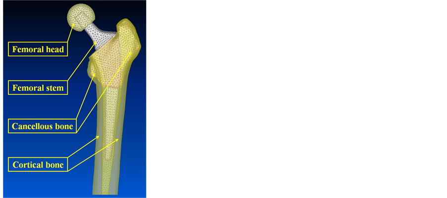
Figure 1. Mesh of the FE model used for the study of thefemur-cementless prosthesis coupled system: DePuy Corail®.
vided into two regions, corresponding respectively to the cortical and the cancellous zones. The femoral head and femoral stem are tied together. The femur is fully constrained at its distal part. Frictional contact at the bone-implant interface is taken into account, leading to nonlinear behaviour.
The position of the femur reproduces the standing position in vivo. The applied force is vertical and is progressively increased to a maximum value corresponding to the maximum load during a walk cycle of a 75 kg person in the unilateral compression position. The numerical results obtained are validated by comparison with in vitro test results [18].
2.2. Uncertain Parameters of the Model
Until now, all the quantities appearing in Equation (10) (i.e. the operator K and the vectors d and f) have been supposed to be deterministic, that is to say not affected by uncertainties.
We now assume that the known prescribed conditions vector f is deterministic and that two mechanical parameters of the operator K are uncertain: the Young’s modulus of the cancellous bone and the coefficient of friction at the interface between the cancellous bone and the femoral stem, respectively denoted  and
and .
.
Therefore K is uncertain through these two parameters. Let  be the vector of
  gathering them. By hypothesis, K depends on
 . Consequently, from Equation (10), the unknown vector
  also depends on
  and is therefore uncertain.
2.3. Control Variable and Associated Failure Criterion
Formally, the solution to Equation (10) can be written:
 (14)
(14)
where  is a nonlinear operation from
  into
into  such that:
 (15)
(15)
A control variable is a real variable, for example a scalar displacement (or a stress, or a strain) at a particular point of the studied mechanical system, whose value must be controlled within the framework of the reliability analysis of the system.
In this work, the chosen control variable is the Euclidean norm of maximum relative displacement between the femoral stem and the cancellous bone.
Let  be such a variable. It depends on the unknown
  through a relationship of the form:
 (16)
(16)
where C is a known function from  into
into , called observation operator. Inserting Equation (14) into Equation (16) yields:
 (17)
(17)
where  is also a known function from
  into
into . As a result,
  can also be viewed as a function of
 . Note that the functions C and D are known, in the sense that they are described by known numerical models.
As seen in Section 2.2, the mechanical operator  depends on the uncertain vector parameter
 . As a result, its inverse
  also depends on
 , as does the function
 , as can be seen from Equation (17). Indicating this fact by the new notation
  and
and  in the place of
  and
and , Equations (14) and (17) become:
 (18)
(18)
and, since  is a constant vector of
 , can be rewritten:
 (19)
(19)
where  is a function from
  into
into  and
and  is a function from
  into
into , such that
 :
:
 (20)
(20)
Let  be a given admissible value of
 , called the failure threshold, and let
  be the real variable such that:
 (21)
(21)
Such a variable is called the safety margin associated with the control variable , and its sign defines two fundamental states for the mechanical model: the safe state if
  and the failure state if
 . The value
  characterizes a limit situation called the failure limit state. According to Equation (19),
  can be rewritten:
 (22)
(22)
where  is a function from
  into
into  called the limit state function of the mechanical model. This function defines three specific subsets of
 :
:
 (23)
(23)
 (24)
(24)
 (25)
(25)
which verify:
 (26)
(26)
and which are respectively called the safe domain, the failure domain and the limit state curve.
The condition  defining the failure state is the failure criterion associated with the control variable
  and its limit value
 . The failure domain
  is the geometric representation of this criterion.
Let us note that, since the function  is only known numerically (through the finite element model described in Section 2.1), the sets
 ,
,  and
and  can only be determined numerically.
3. Probabilistic Modelling
In the following, all the considered random variables (RV) are assumed to be defined on the same probability space , where
  is a sample space,
  is a
is a  -algebra of subsets of
  and
and  is a probability on
 .
.
3.1. Stochastic Modelling of the Uncertain Parameters
In order to take into account the random variability of the uncertain parameters  (the Young’s modulus of the cancellous bone) and
  (the coefficient of friction between the cancellous bone and the femoral stem), these two parameters are modelled as continuous RVs, denoted
  and
and  respectively.
The continuous  -valued random vector
  gathering these two scalar RVs is the probabilistic model of the uncertain vector parameter
 . In view of the intended numerical applications, this random vector is assumed to satisfy the following hypotheses:
(H1) Its components  and
and  are independent.
(H2) They both follow the same type of probability distribution.
(H3) Three types of probability distribution are admissible for these components: uniform, truncated Gaussian and truncated lognormal.
Concerning these hypotheses, we can make the following remarks:
(R1) Let ,
,  and
and  be the probability density functions (pdf) of
 ,
,  and
and  respectively. Then, from (H1):
 , that is,
 :
:
 (27)
(27)
(R2) From (H2) and (H3) the densities  and
and  are both uniform, or truncated Gaussian or truncated lognormal.
(R3) In connection with (H3), let  be a scalar continuous RV with pdf
 . Then
  is said to follow:
a) an uniform distribution with support ,
,  , if:
, if:
 (28)
(28)
b) a truncated Gaussian distribution with mean , standard deviation
  and support
 ,
,
 , if:
, if:
 (29)
(29)
where  is the indicator function of
  (i.e.
(i.e.
 if
if  and
and  if
if ),
),
 is the interval
 ,
,  , and
, and ,
,  are the solutions of the nonlinear system:
 (30)
(30)
in which:
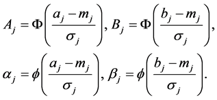
where  and
and  are respectively the one-dimensional standard Gaussian pdf and the one-dimensional standard Gaussian cumulative distribution function, such that:
 (31)
(31)
c) a truncated lognormal distribution with mean , standard deviation
  and support
 ,
,
 , if:
, if:
 (32)
(32)
where  is the interval
 ,
,  , and
, and ,
,  are the solutions of the nonlinear system:
 (33)
(33)
in which:

3.2. Safe and Failure Events
Equations (19) and (22) show that when the uncertain vector parameter  is modelled as a random vector
 , the control variable
  and the safety margin
 , which depend on
 , become scalar RVs. Let
  and
and  be respectively these RVs. They are such that:
 (34)
(34)
and are both defined on the probability space .
.
Naturally, it is assumed here that the definition domains of  and
and  (which are coincident according to Equation (22)) contain the support of the probability distribution of
 .
.
In this random context, the safe state and the failure state are defined by two events, the safe event  and the failure event
 , such that:
 (35)
(35)
 (36)
(36)
and which verify:
 (37)
(37)
Es is the event associated with the safe domain Ds and Ef is the event associated with the failure domain Df.
4. Reliability Analysis
4.1. Fundamental Objective
The fundamental objective of reliability analysis [19] is to calculate the probabilities that the events  and
and  will occur, that is
  and
and . These probabilities are given by:
 (38)
(38)
and, according to Equation (37), satisfy:
 (39)
(39)
where  and
and .
.
From Equation (39),  is known as soon as
  is known and vice versa. That is why in this work our attention is only focused on
 , called the failure probability and denoted
  in the following. This probability can be rewritten:
 (40)
(40)
and its calculation requires the use of a numerical procedure. For the numerical applications treated in this study, we have chosen a Monte Carlo method ([19-21]).
4.2. Standard Formulation
In the classical reliability processes [19], it is customary to transform the initial formulation into a standard formulation in which the vector of random parameters follows a standard Gaussian distribution. This leads in our case to the construction of a regular transformation , with inverse
 , such that the random vector
  can be written:
 (41)
(41)
where  is a
is a  -valued standard Gaussian random vector defined on
 .
.
Once this transformation has been constructed, the failure event can be expressed in terms of  as follows:
 (42)
(42)
where  is a mapping from
  into
into  such that,
 :
:
 (43)
(43)
From Equation (32), the failure probability is then given by:
 (44)
(44)
where ,
,  ,
,  is the subset of
  such that:
 (45)
(45)
And  is the bidimensional standard Gaussian pdf, given by:
 (46)
(46)
Note that Equation (44) can also be obtained by carrying out the variable change  in Equation (40).
The set  is the failure domain in the standardized
  -space, that is in the space (identified with
 ) of the
  random vector’s realizations. Its complementary in
 , that is the subset
 , and the common boundary between
  and
and , that is the curve
 , are respectively the safe domain and the limit state curve in this standardized space (Figure 2).
Equation (44) represents the standard formulation of the reliability problem. To estimate this integral, three Monte Carlo methods were used: the crude direct method and two more refined methods, based respectively on the importance sampling technique and the directional simulation technique ([19-21]).
Such a formulation is completely defined as soon as transformation  is known, and the latter only depends on the probability distribution of the random vector
 . As the components
  and
and  of
of  are assumed independent, this transformation is of the form:
 (47)
(47)
where ,
,  , is the
  -th coordinate of T and
 ,
,  , is a mapping from
  into
into where
where  is the definition domain of the pdf
  of
of .
.
We give below the expression of transformation  for each of the three distributions considered for
  (see Section 3.1, bearing in mind that
  and
and  are both assumed to follow the same type of probability distribution):
a) ,
,  , follows a uniform distribution with support
 ,
, :
:
 (48)
(48)
b) ,
,  , follows a truncated Gaussian distribution with mean
 , standard deviation
  and support
 ,
, :
:
 (49)
(49)
where  is the solution of the system (30).
c) ,
,  , follows a truncated lognormal distribution with mean
 , standard deviation
  and support
 ,
,
 :
:
 (50)
(50)
where  is the solution of the system (33).
Note that the fact that  and
and  are both assumed to follow the same type of probability distribution is not a loss of generality. It is a simple working hypothesis, which could be changed without any incidence on the proposed methodology.
4.3. Hasofer-Lind Index
The Hasofer-Lind index  ([19,22]) is a reliability indicator whose calculation is easier than that of failure probability
 . It is defined in the standardized
  -space as follows:
 (51)
(51)
where  denotes the usual Euclidean distance between the origin point
  and the failure domain
 . Such an index is thus given by:
 (52)
(52)
where  denotes the canonical Euclidean norm on
 .
.
The Rackwitz-Fiessler algorithm ([23,24]) is well suited to solving the constrained nonlinear optimization problem (52) and it was chosen to treat the numerical applications presented in Section 5. Note that for these applications the problem (52) has a unique solution. The solution point:
 (53)
(53)
such that , is called the design point, or
 -point, and is located on the boundary
  of
of 
(Figure 2). If  denotes the vector of
whose components  and
and  are the coordinates of
  (
( is the position vector of
 ), then
  is given by:
 (54)
(54)
where  is the limit state function defined by Equation (43),
  is its gradient (assumed to exist at point
 ), and
  is the canonical Euclidean inner product on
 .
.
4.4. FORM Approximation [19,22,23]
This approximation (FORM means First-Order Reliability Method) consists of replacing the failure domain  by the half-space:
 (55)
(55)
where  is the First-Order Taylor Approximation of
  at point
 , such that:
 (56)
(56)
whose graph  is a straight line tangent to
  at
at  (Figure 2).
The failure probability (44) is then approximated by:
 (57)
(57)
and a simple calculation gives:
 (58)
(58)
where  is given by Equation (54).
4.5. SORM Approximation [19,24]
This approximation is a refinement of the previous method (SORM means Second-Order Reliability Method), which is based is based on the replacement of the failure domain  by the set:
 (59)
(59)
where  is the Second-Order Taylor Approximation of
  at point
 , that is the quadratic function given by:
 (60)
(60)
whose graph  is a second-order curve tangent to
  at
at  (Figure 2). In Equation (60),
  is the Hessian operator associated with
  and is assumed to exist at point
 .
.
Using this substitution, the failure probability (44) is then approximated by:
 (61)
(61)
and this integral can be evaluated by using approximate formulas, such as the Breitung asymptotic formula [25]:
 (62)
(62)
or the Hohenbichler asymptotic formula [26]:
 (63)
(63)
is an improvement of the previous one. In these formulas,  is the curvature of the limit state curve
  at
at ,
,  and
and  are the functions given by Equations (31), and the following conditions are assumed to be verified:
 ,
, .
.
5. Numerical Experiments
The numerical applications presented in this section concern the model of cementless hip prosthesis described in Section 2.1 and aim at estimating its reliability in various situations, either through the Hasofer-Lind index  (calculated from the Rackwitz-Fiessler algorithm) or by means of the failure probability
  (estimated from Monte Carlo simulations or by using the FORM and SORM approximations). All these methods have been implemented by the authors. We recall that the boneprosthesis system is considered as reliable if the Euclidean norm of the maximum relative displacement between the femoral stem and the cancellous bone do not exceed a given admissible value
  (the failure threshold).
5.1. Influence of Probability Distributions and Scatterings
The purpose of this application is to highlight the influence of distributions and scatterings of random parameters on bone-prosthesis system reliability, expressed in terms of the Hasofer-Lind index .
.
For this,  and
and  are assumed to be independent with fixed means
  and variable coefficients of variation
 , and the three following cases are considered:
(C1)  and
and  are uniformly distributed on the intervals
  and
and  respectively(C2)
  and
and  are truncated Gaussian with supports
  and
and  respectively(C3)
  and
and  are truncated lognormal with supports
  and
and  respectivelywhere in each case, for
 :
:
 (64)
(64)
The chosen values for ,
,  and the failure threshold
  are:
are:
 (65)
(65)
For the coefficients of variation  and
and , which quantify the scattering of
  and
and  respectively, three values are considered in each
  case according to the following strategy:
1)  is fixed to its reference value
  and
and  successively takes the values
 ,
,  ,
, ;
;
2)  is fixed to its reference value
  and
and  successively takes the values
 ,
,  ,
, .
.
The results obtained are summarized in Table1 In each case, we can see the significant effect of the coefficients of variation on the index . We can also observe that the effect of
  (coefficient of variation of the coefficient of friction) is greater than that of
  (coefficient of variation of the Young’s modulus of the cancellous bone). Finally, we can point out that the probability distributions of
  and
and  have a minor influence on
 .
.
5.2. Influence of Truncation Lengths
In this application, the random parameters  and
and  are assumed to be independent and distributed according to truncated distributions with variable supports and constant first two moments. Under this assumption, the objective is to evaluate the effect of the support length of each distribution (so-called truncation length) on the reliability of the hip prosthesis expressed in terms of the Hasofer-Lind index
 .
.
The supports  and
and  of the distribution of
  and
and  are chosen of the form:
 (66)
(66)
where  and
and  are strictly positive non-dimensional coefficients controlling the length of the supports. To highlight their influence on
 , four situations are considered:
(TG1)  and
and  are truncated Gaussian,
  and α2 successively takes the values
 ,
,  and
and (TG2)
(TG2)  and
and  are truncated Gaussian,
  and
and  successively takes the values
 ,
,  and
and (TLN1)
  and
and  are truncated lognormal, α2 = 2.5 and
  successively takes the values
 ,
,  and
and (TLN2)
  and
and  are truncated lognormal, α1 = 2.5 and
  successively takes the values
 ,
,  and
and .
.
The chosen values for the statistics , j = 1,2and the failure threshold
  are the following:
 (67)
(67)
The results obtained are listed in Table2 First we can see that the behaviour of  with respect to the truncation lengths depends on the nature of the considered probability distributions. Indeed, in the truncated Gaussian case this behaviour is non-monotonous (
 decreases then increases) in each considered situation (TG1 and TG2), while in the truncated lognormal case, it is either increasing monotonous (situation TLN1) or decreasing monotonous (situation TLN2). In each case, however, the influence of the truncation lengths on
  is not very significant.
5.3. Influence of the Failure Threshold
In this section, we study the influence of the failure threshold  on the reliability of the prosthesis, again using the Hasofer-Lind index
  as a reliability indicator.
To this end, the random parameters  and
and  are assumed to be independent and uniformly distributed with means and standard deviations given by Equation (67); five values are successively considered for the failure threshold
  (in
(in ): 270, 275, 28 0, 285, 290.
The obtained values of  are given in Table 3 which also contains, for information, the corresponding values for the FORM approximation
  of failure probability, given by Equation (58).
We can first observe that the values of  are quite low for all the considered values of
 , which are nevertheless common values for this threshold. This comes quite obviously from the chosen values for the coefficients of variation of
  and
and , which are relatively high
 . We can also underline that these results are logical in the sense that
  increases as
  increases. It is interesting, moreover, to note that this increase is quasi-linear over the range of the considered
  values.
5.4. Comparison of Various Approximations of Pf
In this application we consider the same example as in the previous application (see Section 5.3), and for each value of the failure threshold  we compare the FORM and SORM approximations
  and
and  of
of  (given by Equations (58) and (63) respectively) with the target value of this probability, obtained by using the crude Monte Carlo method taken as the reference method.
Estimating  from the latter requires here the simulation of
  realizations
 , of the standard Gaussian vector
 , then, for each simulated realization
 , the calculation of the corresponding value
  of the limit state function
 . Such an estimation requires thus
  finite element calculations. This is why two other less expensive Monte Carlo methods were used: one based on the importance sampling (IS) technique, the other on the directional simulation (DS) technique ([19- 21]).
The values of  given by these two improved Monte Carlo methods and by the crude Monte Carlo method are respectively denoted
 ,
,  and
and . The comparison of
  and
and  with
with  is shown in Table4 Table 5 gives, for
 , the number of finite element calculations required by the Monte Carlo methods based on the IS and DS techniques to provide the same value for
  as that given by the crude Monte Carlo method (i.e.
 ).
).
The results obtained show first that  and
and  are poor approximations of
 . They also show that
  is not a significant improvement on
 . This can be explained by the fact that the local approximations
  and
and  of the limit state curve
  (Figure 2) are not accurate enough to adequately represent
  in a sufficiently large neighbourhood of the design point
 . The results in Table 5 confirm that the Monte Carlo methods based on the IS and DS techniques are more efficient than the crude Monte Carlo method. We can also observe that the method based on the DS technique is less time-consuming, and therefore more efficient, than the one based on the IS technique.

Table 5. Number of finite element (FE) calculations required by the Monte Carlo methods based on the IS and DS techniques to provide the same value for  as that given by the crude method.
6. Conclusions
The aim of this paper was to present a methodology to enable the prediction in a probabilistic context of the primary stability of cementless hip prostheses in the presence of uncertainties. Based on a reliability approach, this methodology supposes the numerical model describing the mechanical behaviour of the prosthesis-cancellous bone couple, the probabilistic models of uncertain parameters and the failure criterion expressing the loss of stability of the prosthesis to be known. The underlying mechanical problem is a classical problem of contact with friction between two three-dimensional deformable bodies: a Depuy Corail® prosthesis is implanted without cement in a femur. This problem is solved using a finite element model based on Bathe’s formulation. Due to their variability in the literature, we chose to consider the Young’s modulus of the cancellous bone and the coefficient of friction between the cancellous bone and the femoral stem as uncertain parameters. They were modelled as random variables, assumed successively to be uniform, truncated Gaussian and truncated lognormal. Finally, failure was defined as the exceeding of a given limit value by the maximum relative displacement between the femoral stem and the cancellous bone. The reliability of the coupled system was estimated using two indicators: the Hasofer-Lind index and the failure probability. The first was calculated using the RackwitzFiessler optimization algorithm. The second was estimated first by using approximate formulas derived from FORM and SORM approaches, then by means of three Monte Carlo methods: the crude Monte Carlo method, the method based on the importance sampling technique and that based on the directional simulation technique.
The presented numerical applications have shown the relevance of the proposed methodology and given an indication of its great potential in the field of prosthesis reliability. A different failure criterion could be envisaged, such as the acceptable maximum stress or the optimization of the contact area, for instance.
This methodology has been presented in the case where only two parameters are uncertain. It is clear, however, that its validity and its operational capacity would not be compromised by an increase in the number of uncertain parameters. This personal probabilistic model enables clinicians to compare the primary stability of cementless prostheses, and to choose the optimal implant design while taking into account uncertainties in the model input data.
Acknowledgements
This work was financially supported by the Conseil Général de l’Allier and Society DePuy France.