Global Stability Analysis of a Delayed SEIQR Epidemic Model with Quarantine and Latent ()
1. Introduction
Many people have been paying attention to the study of some epidemics, and have accumulated a lot of experience. By establishing reasonable mathematical models, they put forward the measures which controlled the spread of epidemics effectively. And many scholars researched specific diseases and considered the diseases with incubation period, recovery time, quarantine and so on [1-6]. So many epidemics were controlled. Generally speaking, when epidemics spread, there are many kinds of delays, which include immunity period delay [7-9], infectious period delay, incubation period delay. In [10], Enatsu et al. studied stability analysis of delayed SIR epidemic models with a class of nonlinear incidence rates, at the same time, they proved disease-free equilibrium was globally asymptotically stable and endemic equilibrium was permanent under certain conditions. At the same time, global stability of an SIR (where S, I, R denote the number of susceptible individuals, infectious individuals, recovery individuals) epidemic model with constant infectious period was studied by Zhang et al.
[11], they showed the endemic equilibrium was globally asymptotically stable with appropriate Lyapunov functions. And in [12], Gao et al. discussed pulse vaccination of an SEIR (E denote the number of exposed individuals) epidemic model with delay and bilinear incidence. Meanwhile, impulsive vaccination of SEIR epidemic model with time delay and nonlinear incidence rate was researched by Zhao et al. [13], and showed the pulse system that was similar to the pulse system with bilinear incidence rate. Besides, on the basis of [13], Xu and Ma introduced the saturated incidence rate. Meanwhile, they showed disease-free equilibrium and endemic equilibrium were globally asymptotically stable under certain condition in [14]. However, in addition to the bilinear incidence rate, nonlinear incidence rate and saturated incidence rate, there were some scholars who studied the non-monotone incidence. For example, an SIRS epidemic model with pulse vaccination and non-monotonic incidence rate was discussed by Zhang et al. [15], and they proved the disease-free equilibrium and endemic equilibrium were asymptotically stable under certain conditions. Besides, some scholars studied a delayed SEIQR (Q denote the number of quarantined individuals) epidemic model with pulse vaccination and the quarantine measure, and they showed that the disease-free equilibrium of the system was globally attractive and endemic equilibrium was permanent under certain conditions. In this paper, we study a delayed SEIQR epidemic model without pulse on the basis of [14,16].
The organization of this paper is as follows: In Section 2, SIQR epidemic model and its basic reproduction number and existence of equilibrium are given. In Section 3, the local stability of endemic equilibrium and disease-free equilibrium is showed by using Hurwitz criterion. By using suitable Lyapunov functions and LaSalle’s invariance principle, we prove the disease-free equilibrium is globally asymptotically stable when the basic reproduction number is less than unity and the endemic equilibrium is globally asymptotically stable when the basic reproduction number is greater than unity. At the same time, the system with the nonlinear incidence rate is discussed in Section 3. In Section 4, presents the numerical simulations of the system followed by a conclusion in Section 3. At last, a brief discussion is given in Section 5 to conclude this work.
2. Establishment of the Model
We establish the following SEIQR epidemic model, Here  represents the number of individuals who are susceptible to disease, that is, who are not yet infected at time t.
  is the number of individuals who are infected but hardly infectious. So we think they can’t infect other people, but they need to be quarantined.
  represents the number of infected individuals who are infectious and are able to spread the disease by contact with susceptible individuals.
  is the number of infectious individuals who are quarantined at time t.
  represents the number of recovered individuals at time t.
 (1)
(1)
The initial conditions for system (1) are

And the feasible region of the model with the initial conditions above is

Here, we presume that

It is easy to show that  is positively invariant with respect to system (1).
Where all the parameters are positive constants,  is the recruitment rate of the susceptible population,
  ,
, 


 are the natural death rate of the susceptible, exposed, infectious, quarantine and recovered respectively,
  is the disease transmission coefficient,
  is the death rate due to disease without quarantine,
  is the death rate due to disease after quarantine,
  is the recovery rate after quarantine,
  is the recovery rate without quarantine,
  ,
,  are quarantine rate of
 ,
,  respectively,
  is the recovery rate of
  and
and  is the latent period of the epidemic.
Because the variables R and Q do not appear in the first three equations in system (1), we further simplify system (1) and then obtain the following model
 (2)
(2)
In this paper, we are concerned with system (2).
The initial conditions for system (2) are
And the feasible region of the model with the initial condition above is

Here, we presume that

It is easy to show that  is positively invariant with respect to system (2).
According to the practical significance of the epidemic model, system (2) always has a disease-free equilibrium

Denote the basic reproduction number of system (2)

Define  If the basic reproductive number
  system (2) has an unique endemic equilibrium

3. The Stability of Equilibrium
In this section, we discuss the local stability of endemic equilibrium and disease-free equilibrium of system (2) by analyzing the corresponding characteristic equations respectively. By defining reasonable Lyapunov functions, we resolve the global dynamics of equilibriums without requiring any extra conditions. In addition, system (2) with nonlinear incidence is studied.
3.1. Stability of Disease-Free Equilibrium
Theorem 3.1.1. If , the disease-free equilibrium
  of system (2) is locally asymptotically stable for any
  in
in . If
. If , it is unstable for any
  in
in .
.
Proof. The characteristic matrix at the disease-free equilibrium 

When  the characteristic equation at the disease-free equilibrium
  of system (2) takes the form
Clearly, system (2) always has two negative real roots

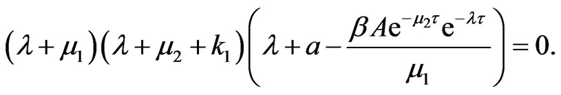
All other roots are given by the roots of equation


Assume 

That is, 
Because 
 which is contradictory. So
  Therefore the disease-free equilibrium
  of system (2) is locally asymptotically stable.
If  let
let

so there is a positive real root at least. The disease-free equilibrium  of system (2) is unstable.
When  it is easy for us to prove the disease-free equilibrium
  of system (2) is locally asymptotically stable.
Theorem 3.1.2. If , the disease-free equilibrium
  of system (2) is globally asymptotically stable for any
  in
in .
.
Proof. For  define a differentiable Lyapunov function


Obviously, 
Calculating the derivative of  along positive solutions of system (2), it follows that

According to the feasible region, 
So
That is,

And when 
While  if and only if,
For all t, it is easy to show that  is the largest invariant subset of the set
  Because of LaSalle’s invariance principle, disease-free equilibrium
  of system (2) is globally asymptotically stable. This completes the proof.
3.2. The Stability of Endemic Equilibrium
Theorem 3.2.1. For any , if
, if  the endemic equilibrium
  of system (2) is locally asymptotically stable in
Proof. The characteristic matrix at the endemic equilibrium 

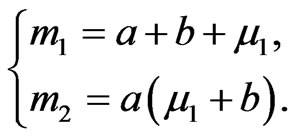
Order 
The characteristic equation at the endemic equilibrium  is
is

Clearly, system (2) always has a negative real root

When  all other roots are given by the roots of equation
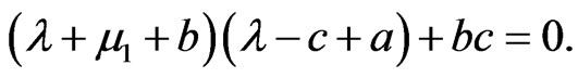
 so
so

So according to Hurwitz criterion, the endemic equilibrium  of system (2) is locally asymptotically stable.
When  all other roots are given by the roots of equation

Simplify, we can get

Let
Then
 (3)
(3)
Let  is the root of Equation (3), on substituting to
  Equation (3), we derive that

Separating real and imaginary parts, it follows that

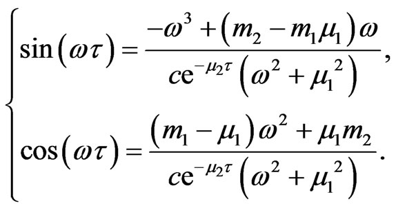
Then we can get

Order

Letting  then Equation (4) becomes

Here

Application of the conclusions of [17], we can know that positive  doesn’t exist. Hence
  also doesn’t exist. There are not pure imaginary roots in system (2). Therefore all the roots have negative real component. So endemic equilibrium
  of system (2) is locally asymptotically stable.
Theorem 3.2.2. If  when
when  the endemic equilibrium
  of system (2) is globally asymptotically stable in
Proof. Define a differentiable Lyapunov function


 both of them are real numbers. The function is positive definite. Calculating the derivative of
  along positive solutions of system (2), it follows that

On substituting  we have

Let 
So  In addition, when
  if and only if
It is easy to show that  is the largest invariant subset of the set
  Because of LaSalle’s invariance principle, the endemic equilibrium
  of system (2) is globally asymptotically stable when
 . This completes the proof.
Theorem 3.2.3. If  when
when  the endemic equilibrium
  of system (2) is globally asymptotically stable in
Proof. For  define a differentiable Lyapunov function

Order

 both of them are real numbers. Let

Then the derivative of  along the solution of system (2) satisfies


Then

Simplify, we can get
Order 
 Besides, when
  if and only if
It is easy to show that  is the largest invariant subset of the set
  Because of LaSalle’s invariance principle, the endemic equilibrium
  of system (2) is globally asymptotically stable when
 . This completes the proof.
3.3. The SEIQR Epidemic Model with Nonlinear Incidence Rate
Zhao et al. studied delay SEIR epidemic model with the nonlinear incidence rate like  in the case of pulse. In this paper, the model without pulse is discussed.

It is easy to show disease-free equilibrium is globally asymptotically stable, endemic equilibrium is locally asymptotically stable. The ways we use are similar to that in system (1), here they are omitted.
4. The Numerical Simulations
In this section, we study system (1) numerically. According to the different datas that can reflect the actual situation, we get the different simulation images to prove our conclusions obviously (Figures 1-9).
Here, according to the different actual situations, while take different parameters, we can get different simulation diagrams of the disease-free equilibrium. At the same time, we find out the disease will die out after much more time when  increases. For example,
Here  see Figure 1.


Figure 1. Simulation diagram of the disease-free equilibrium when .
.
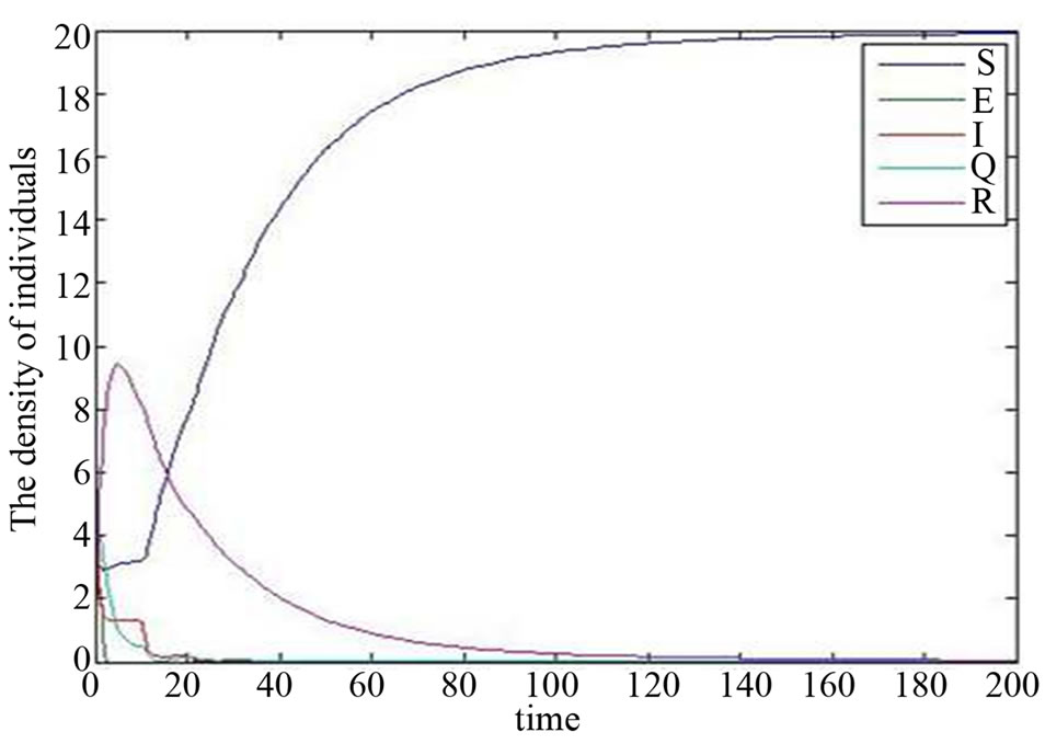
Figure 2. Simulation diagram of the disease-free equilibrium when .
.
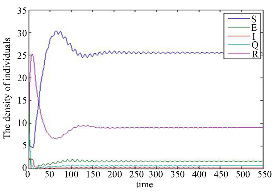
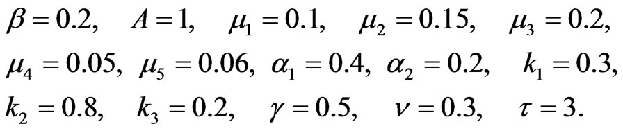
Figure 3. Simulation diagram of the endemic equilibrium when .
.
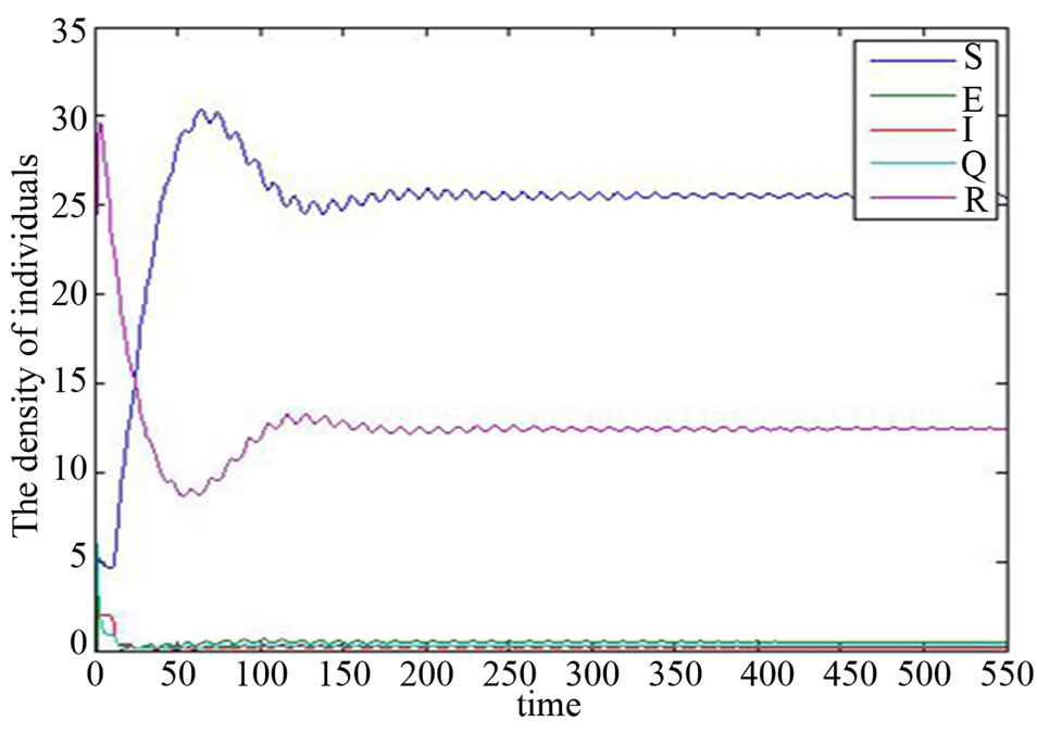
Figure 4. Simulation diagram of the endemic equilibrium when .
.

Figure 5. Simulation diagram of the endemic equilibrium when .
.
Here  see Figure 2.
When take different , we can get different simulation images. In other words, the
  increases when
  increases, which is obvious in Figures 3 and 4. And then it is easy for us to find that how
  effects changing trends of
 ,
,  ,
,  ,
,  ,
, .
.

Figure 9. Simulation diagram of basic reproduction number.

Here  see Figure 3.

Here  see Figure 4.
At last, if the basic reproduction number is much larger and we will get new diagrams. For example, let

Here  see Figure 5.
At the same time, the changing trends of  and
and  are shown in Figures 6 and 7. And the time which
  comes peak will become large as
  increases, the
  will decrease. For example,
  , see Figure 8. In addition, when
  changes,
  will change. And we can find out that when
  That is, disease will be endemic disease while
  see Figure 9.
5. Discussions
In this paper, a kind of a delayed SEIQR epidemic model with the quarantine and latent is studied. Using Hurwitz criterion, the local stability of the disease-free equilibrium and endemic equilibrium of system (2) is proved. For any time delay  we prove the disease-free equilibrium is globally asymptotically stable when the basic reproduction number is less than unity and the endemic equilibrium is globally asymptotically stable when the basic reproduction number is greater than unity by means of suitable Lyapunov functions and LaSalle’s invariance principle. So the delay is harmless to system (2). From the biological point of view, the delay here has no influence on the transmission of diseases. However, in [16], the disease-free equilibrium is periodic and globally attractive. At the same time, the disease will be endemic after some period of time. Above all, we consider that
  is quarantined and can recover in this model, which will effect changing trends of
 ,
,  ,
,  ,
,  ,
, . Here, we take
  as an example to explain that. Meanwhile, the simulation image which
  changes as
  can be obtained and we can find out
  which the basic reproduction number is a unity. Those are useful for us to control epidemics. At last, the conclusions above are verified by numerical simulations.
6. Acknowledgements
This research was supported by the National Science Foundation of China (10471040) and the National Sciences Foundation of Shanxi Province (2009011005-1).
NOTES