Reconstruction of UWB Impulse Train by Parallel Sampling of Cascaded Identical RC Filters ()
1. Introduction
The conventional sampling methods are based on the sequential measurement of signals at equidistant intervals. If the signal contains abrupt changes, such as edges, impulses and other discontinuities, the signal bandwidth is not limited below the Nyquist frequency and the Shannon’s sampling theorem is not warranted. Recently the problem to measure and reproduce non-band limited signals has been widely studied in signal processing society. Excellent articles [1-8] concern on the prefiltering and reconstruction of signals under nonideal sampling constraints. The sampling scheme based on the finite rate of innovation (FRI) recovers a variety of transient signal families, which are not band limited, such as impulses, piecewise linear and amplitude modulated edges.
The measurement and recovery of short term transient signals (Diracs) plays a main role in wireless ultra wideband (UWB) technology, where the information is coded to impulse sequences. The Diracs are fed to an analog circuit, which has a specific impulse response. The purpose of the sampling filter is to lengthen the UWB impulses for equidistant sampling by an analog-to-digital converter. Various methods have been developed for reconstruction of the original signal from discrete samples.
Our research group has introduced a sampling scheme, where the signal is fed to the parallel RC filters, whose outputs are sampled simultaneously [9,10]. A variant of the parallel sampling scheme is tailored for detection of edges [11,12]. The parallel sampling scheme can be applied to reproduce transient signals without ad hoc knowledge of the signal waveform [13]. Recently a multichannel sampling (MCS) arrangement was introduced, where the input signal is modulated by a set of sinusoidal waveforms, followed by a bank of integrators [14]. The MCS yields Fourier series coefficients, which enable the reconstruction of the input signal.
In this framework we introduce a new method for measurement and reconstruction of the impulse trains based on the parallel sampling of the identical cascaded RC filters. We show that the amplitudes and locations of p Diracs can be reproduced from simultaneous measurements of 2p outputs of cascaded identical RC filters. We compare the reconstruction performance of the present method with the MCS arrangement using an analog electronic circuit simulator.
2. Theoretical Considerations
2.1. Sampling of the Impulse Train
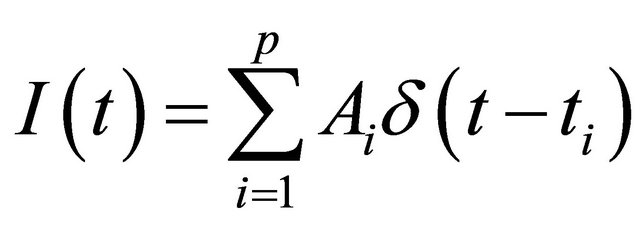
We consider the impulse train consisting of p sequential Dirac distributions
 (1)
(1)
where  are amplitudes and
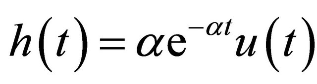
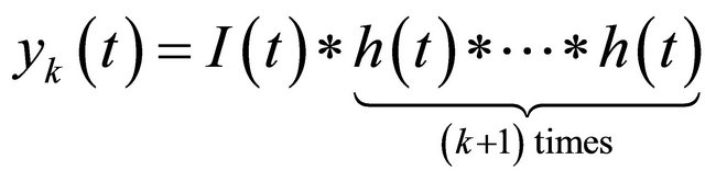
  the time locations. The impulse train is fed to the N identical cascaded RC filters (Figure 1), each having the impulse response
 (2)
(2)
 of the cascaded RC filter network are obtained as where the unit step function
 for
for  and
and  for
for  and
and . The output signals
 (3)
(3)
In Laplace transform domain we have
 (4)
(4)
The inverse Laplace transform then gives
 (5)
(5)
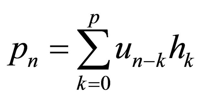
where . Now we can write the convolution integral
 (6)
(6)
The prominent idea in this work is to measure the RC filter outputs  simultaneously at a time
 . By denoting the time difference
  and rearranging we obtain
 (7)
(7)
where the notations  and
and  are used.
2.2. Reconstruction Algorithm
In the following we develop a reconstruction algorithm for the amplitudes and time locations of the Diracs based
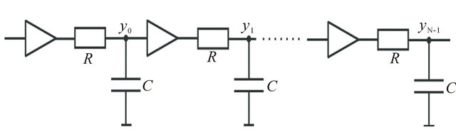
Figure 1. The arrangement for measurement of the impulse train based on the parallel sampling of N cascaded identical RC filters, which are separated by the unity gain buffer amplifiers.
on formulation (7). The z transform of the  sequence with respect to k yields
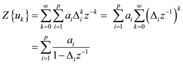 (8)
(8)
Let us define the pole cancellation filter as
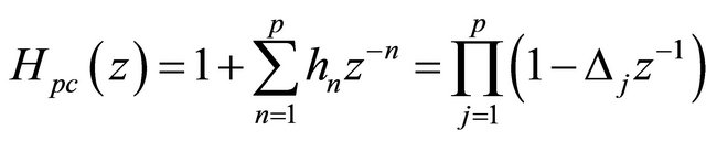 (9)
(9)
and the  polynomial as
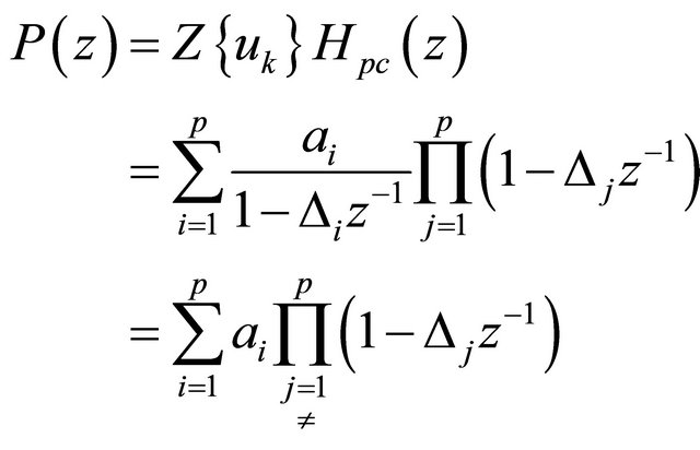 (10)
(10)
Clearly the roots of the pole cancellation filter correspond to the roots of the  polynomial. The impulse response
  of the
  can be computed from convolution
 (11)
(11)
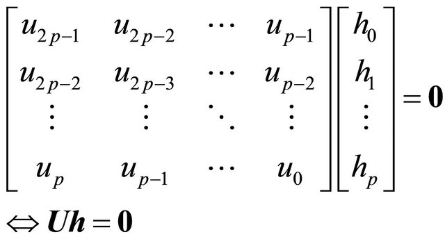
The roots of the  are obtained by setting
  for
for . This yields the matrix/vector equation
 (12)
(12)
We may observe that the solution of the coefficients of the pole zero cancellation filter requires the knowledge of the 2p values of the  sequence. The polynomial
 has roots
 .
.
The time locations of the Diracs are then obtained as . For solution of the amplitudes we may write (7) in matrix/vector form
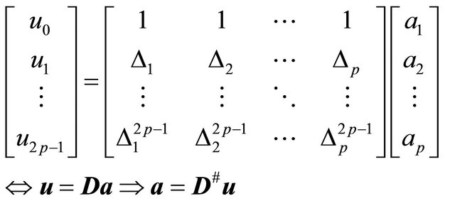 (13)
(13)
where # denotes the pseudoinverse matrix. Now the amplitudes of the impulses are obtained as . To summarize, the reconstruction of p impulses requires the knowledge of the
  sequence. This needs the simultaneous measurement of at least
  samples from the outputs of the cascaded RC filters. An alternative singular value decomposition (SVD) based null space method is presented in Appendix for the solution of the roots of the pole zero cancellation filter (9).
2.3. Noise Cancellation
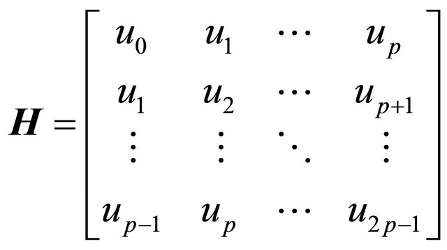
The above formulation (8)-(13) is valid only in noise free situation. The noise was rejected by the singular value decomposition (SVD) based subspace method. Let us construct a Hankel matrix
 (14)
(14)
where the antidiagonal elements are identical. The singular value decomposition of the matrix  is
is , where
  and
and  are unitary matrices.
  is a diagonal matrix consisting of the singular values in descending order. We may decompose
  as
as
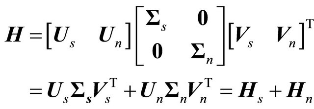 (15)
(15)
 contains the smallest singular values and hence the matrix
  can be considered to belong to the noise subspace. The matrix
  is then related to the noise free signal subspace. The dimension of the signal subspace can be evaluated by several methods [15]. In this work we plotted the logarithm of the singular values in descending order. The logarithmic singular values form clearly separable linear groups. In all cases the dimension of the signal subspace appeared to be p, i.e. the number of impulses. The signal matrix
  is not precisely a Hankel matrix, as some variation occurs in the antidiagonal elements. We reconstructed the noise free Hankel matrix by replacing the antidiagonal elements by their mean values.
2.4. High-Speed Sampling Method
In the case the impulse rate is limited so that only one impulse arrives at the cascaded RC network, the reconstruction algorithm simplifies notably and the sampling of the outputs of the first two RC filters is enough to recover the amplitude and time location of the impulse. Based on (6) we obtain
 (16)
(16)
In practice the outputs of at least three RC filters is advisable to measure, since we may then construct the Hankel matrix  for SVD based noise cancellation.
2.5. Elimination of the Pulse Pile-Up in UWB Transmitter
The practical UWB transmission protocol consists of wireless RF pulses each containing three impulses (Figure 2). The current reconstruction algorithm (12, 13) does not take into account the pulse pile-up effect due to the previous pulses in cascaded RC network. Let us consider the situation in which the UWB pulses are transmitted at constant time intervals  and the parallel sampling of the outputs of the RC network also occurs at
  intervals. By denoting the sampled and normalized outputs by
  and applying (7), we have
 (17)
(17)
contains the output due to the impulses occurring at time interval  reduced by the pile-up signal due to the previous UWB pulses at time interval
 . The approximation in (17) is exact for
 . However, in cases for
  the exponential
  is mainly responsible for the descending tail and the approximation error is negligible.
3. Experimental
The reconstruction algorithm was tested by an extensive simulation study. The cascaded network comprised eight identical RC filters which were constructed using an ana-

Figure 2. The output signal of the cascaded RC filter network comprising of eight cascaded identical RC circuits. Each UWB pulse consists of three Diracs.
log electronic circuit simulator (Spice). The  parameter varied in the range 0.1 - 0.8. In the absence of noise the reconstruction algorithm (12, 13) recovered the amplitudes and time locations of the impulse train consisting of 1 - 4 Diracs with machine precision. When the random noise was added to the input of the network, the algorithm could reconstruct 1 - 3 Diracs with good accuracy, when the SVD based subspace method was applied to noise cancellation. The error in amplitudes varied between 0.8 - 1.2 percent and in time locations 0.3 - 0.7 percent. In the case of four sequential Diracs the reconstruction algorithm yielded inaccurate results or totally failed.
We made a preliminary comparison with the multichannel sampling (MCS) arrangement [14] using the Spice simulation toolbox. In the case of 1 - 3 sequential impulses the performance of the MCS was clearly poorer than the results obtained by the present RC filter network in the presence of noise below SNR < 45 dB, but significantly higher at SNR > 45 dB. In the case of four sequential impulses the performance of the MCS was significantly higher compared with the present reconstruction method in all noise levels.
The cascaded RC network was implemented using metallic foil resistors and low-noise capacitors. Eight RC filters were separated by unity gain buffer amplifiers (Figure 1). The outputs of the RC filters were sampled simultaneously with an eight channel differential 12-bit analog-to-digital converter (ADC) equipped with a sample and hold (S/H) circuit in every channel. For 1 - 3 Diracs the reconstruction error in amplitudes was between 1.1 - 1.4 percent and in time locations 0.6 - 0.9 percent. For four Diracs the reconstruction error was considerably higher, for amplitudes 2.2 - 3.4 percent and for time locations 0.9 - 1.7 percent. In all experimental measurements the SVD based subspace method was used for noise rejection. The high-speed sampling method (16) recovered the amplitudes and time locations of single Diracs with good accuracy using three cascaded RC filters. The amplitude error was between 0.6 - 1.3 percent and the error in time locations 0.1 - 1.1 percent.
The reconstruction of Diracs using the SVD based null space method (Appendix) gave almost identical results, which are not repeated here. The slight difference is probably due to that the matrices  in (14) and
  in (17) are different.
4. Conclusions
In our previous work [9] we introduced a novel sampling scheme based on parallel RC filters, where the outputs were measured simultaneously. A disadvantage in the practical construction of the parallel RC network comes from the precise adjustment of the time constants of the RC circuits. For N parallel RC circuits the  parameter must obey the condition
 . On the contrary, in present cascaded network all RC filters and buffer amplifiers are identical and much simpler to implement in integrated VLSI circuits. Compared with the previous FRI methods, which are based on the sequential sampling, the outputs of the parallel RC filters are sampled only once per UWB pulse, which contains a restricted number of impulses (Figure 2). This eliminates the need for high frequency analog-to-digital converters (ADCs), since the UWB pulse repetition rate can be adjusted to match the ADC’s performance.
The formulation of the reconstruction algorithm was warranted by extensive simulation study using Spice toolbox. In the presence of noise the SVD based noise cancellation method had to be applied. The computational complexity of the SVD algorithm is , which restricts the real-time applications of the present method to a relatively low transmission rate. However, since the information is coded to both the amplitude and the time locations of the Diracs, the number of transmitted pulses can be significantly lower compared with the conventional UWB methods. As an advantage lower number of transmitted pulses reduces the RF radiation load.
We showed in Spice simulation study that in noise free conditions the p Diracs can be reconstructed from sampling the outputs of the 2p cascaded identical RC filters. In the presence of noise this theoretical “2p rule” is not valid and it seems evident that preferable “2p + 1 rule” should be applied.
The high-speed method (16) suits best for reconstruction of single Diracs, whose amplitudes are quantized to only a few levels. For example the impulses with 15 discrete levels can be produced by a 4-bit digital-to-analog converter, which the method reproduces perfectly.
In MCS arrangement the signal is modulated by a set of sinusoidal waveforms, followed by a bank of integrators [14]. The MCS produces Fourier series coefficients, which enable to reconstruct the input signal. However, the MCS is much more complex compared to the circuit consisting of the cascaded identical RC filters. The Spice simulation study revealed that the MCS outperforms the present approach at high noise level, SNR over 45 dB, but inferiors at lower noise environment. To the best of our knowledge the hardware for the implementation of the MCS is not yet available. Hence, in this moment this figure is based only on a simulation study.
In most of the UWB devices information is transmitted by monocycle Gaussian pulses. The FCC restricted the UWB frequency band between 3.1 - 10.6 GHz in year 2002 [16]. The Gaussian pulse train does not meet this constraint and other pulse shapes have been introduced to meet the FCC criteria, e.g. the family of the orthogonal UWB pulse waveforms [17,18]. The fast digital-to-analog converters (DACs) can produce UWB pulses, where the information is coded via orthogonal base vectors and reproduced by matrix/vector computation.
In this work we have concentrated on the UWB communication device, which transmits pulses consisting of most 1 - 3 impulses. The information is coded to the amplitudes and time locations of the Diracs. Such pulse generators are relatively easy to implement in VLSI [19]. Following [18] the impulse train can be designed so that its spectral density spectrum coincides with the FCC criteria.
5. Acknowledgements
This work was supported by the National Technology Agency of Finland (TEKES).
Appendix
SVD Based Null Space Solution
Let us write the convolution (11) in the matrix/vector form
 (18)
(18)
In the following we describe the singular value decomposition (SVD) based null space solution of the unknown vector  in (18). The SDV of the
  matrix in (18) yields
 (19)
(19)
where matrices  and
and  contain the left and right singular vectors (column vectors) and matrix
  the singular values in descending order. Matrices
  and
and  are unitary, i.e.
  and
and , where
  is the identity matrix. Applied to (19) we obtain
 , which yields
 (20)
(20)
Finally we may write
 (21)
(21)
for . Equation (21) forms the basis for the SVD based null space method. By searching very small singular value
 , the right singular vector
  equals vector
  in (18) yielding the solution for the roots of the pole cancellation filter (9). In the presence of noise the dimensions of the
  and
and  matrices should be selected so that there appears only one tiny singular value. This can be also achieved by zeroing the rest of the tiny singular values. It should be pointed out that the SVD based null space method does not yield the coefficients of the pole zero cancellation filtering (9) in normalized form, i.e.
 . However, we may apply post normalization as
  for
for .
.