1. Introduction and Preliminaries
In last years, many authors have studied  -analogues of the binomial distribution (see among others [2-4]). Specifically, Kemp and Kemp [3] defined a
  -analogue of the binomial distribution with probability function in the form
 (1)
(1)
where  by replacing the loglinear relationship for the Bernoulli probabilities in Poissonian random sampling with loglinear odds relationship. Also, Kemp [4] defined (1) as a steady state distribution of birth-abort-death process.
Futhermore, Charalambides [2] considering a sequence of independent Bernoulli trials and assuming that the odds of success at the ith trial given by

is a geometrically decreasing sequence with rate q, derived that the probability function of the number X of successes up to n-trail is the q-analogue of the binomial distribution with p.f. given by Equation (1).
For q constant, the q-binomial distribution has finite mean and variance when .Thus, the asymptotic normality in the sense of the DeMoivre-Laplace classical limit theorem did not conclude, as in the case of ordinary hypergeometric series discrete distributions. Also, asymptotic methods—central or/and local limit theorems—are not applied as in Bender [5], Canfield [6], Flajolet and Soria [7], Odlyzko [8] et al.
Recently, Kyriakoussis and Vamvakari [1], for q constant, established a limit theorem for the q-binomial distribution by a pointwise convergence in a q-analogue sense of the DeMoivre-Laplace classical limit theorem. Specifically, the pointwise convergence of the q-binomial distribution to a Stieltjes-Wigert continuous distribution was proved. In detail, transferred from the random variable  of the q-binomial distribution (1) to the equal-distributed deformed random variable
 , then, for
  the q-binomial distribution was approximated by a deformed standardized continuous Stieltjes-Wigert distribution as follows
 (2)
(2)
where  such that
  with
with  constant and
  and
and  the mean value and variance of the random variable
  respectively. To obtain the above pointwise convergence (2), a qanalogue of the well known Stirling formula for the
  factorial
  has been provided.
In statistical mechanics and in computer science such as in probabilistic and approximation algorithms, applications of the  -binomial distribution involve sequences of independent Bernoulli trials where in the geometrically decreasing odds of success at the
  th trial, the rate
  is considered to be a sequence of
  with
with  as
as  In this work, under this consideration, a question arises. How this assumption affects the continuous limiting behaviour of this q-binomial distribution?
The answer to this question is given in this manuscript by establishing a deformed Gaussian limiting behaviour for the  -Binomial distribution is proved. The proofs are concentrated on the study of the sequence
  and the parameters of the considered distribution as sequences of
 . Further, figures using the program MAPLE are presented, indicating the accuracy of the established distribution convergence even for moderate values of
 .
.
2. Main Results
2.1. An Asymptotic Expansion of the q(n)-Factorial Number of Order n with  as
as 
To initiate our study we need to derive an asymptotic expansion for  of the q-factorial number of order
 (3)
(3)
where  with
with  as
as  and
and
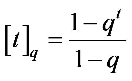 , the q-number t.
The derived estimate for the  -factorial numbers of order
 , is based on the analysis of the
  -Exponential function
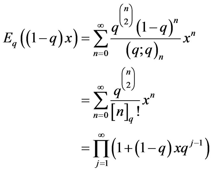 (4)
(4)
which is the ordinary generating function (g.f.) of the numbers .
.
Rewriting  as follows
 (5)
(5)
where
 (6)
(6)
because of the large dominant singularities of the generating function , a well suited method for analyzing this is the saddle point method.
Using an approach of the saddle point method inspired from [9-12] and [1], the following theorem gives an asymptotic for the  -factorial number of order n.
Theorem 1. The q-factorial numbers of order ,
, , where A)

or B) 
have the following asymptotic expansion for 

(7)
where  is a positive integer,
  is the real solution of the equation

and
 (8)
(8)
with  the partial Bell polynomials,
  the Stirling numbers of the second kind and
 .
.
Proof. We shall study the asymptotic behaviour of the  -factorial numbers of order
 ,
,  , by expressing them via Cauchy’s integral formula that gives the coefficients of a power series:
 (9)
(9)
where the contour of integration is taken to be a circle of radius . This integral will be estimated with the saddle point method. The saddle point is defined by the equation
 . It turns out that it is convenient to switch to polar coordinates, setting
 . Then the original integral becomes
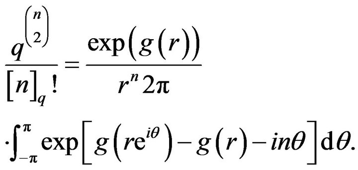 (10)
(10)
In accordance with the saddle point method principles, we choose the radius  to be the solution of
 . Setting
  with a Maclaurin series expansion about
  we have
 (11)
(11)
where
 (12)
(12)
and
 (13)
(13)
where

The absence of a linear term in  indicates a saddle point. The function
  is unimodal with its peak at
 .
.
An estimation of the -factorial numbers of order
  with
with  defined by conditions (A) or (B) should naturally proceed by isolating separately small portions of the contour (corresponding to
  near the real axis) as follows.
A) For  with
with  we set
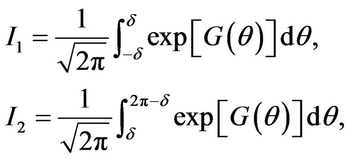 (14)
(14)
and choose  such that the following conditions are true (see [12]):
C1) , that is
C2) , that is
 where “
 ” means “much smaller than”. A suitable choice for
  is
is .
.
As  decreases in
 ,
,
 (15)
(15)
We will show in the sequel that from C1) and C2) it follows that  is exponentially small, being dominated by a term of the form
 .
.
Indeed we have


 (16)
(16)
But

or
 (17)
(17)
For  with
with  we get
 (18)
(18)
From which we find that
 (19)
(19)
Thus, by C1),  has been taken large enough so that the central integral
  “captures” most of the contribution, while the remainder integral
  is exponentially small by (19).
We now turn to the precise evaluation of the central integral . We have
 (20)
(20)
where
 (21)
(21)
Note that  as
as , since

where  a positive constant.
B) For  with
with 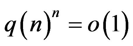 we set
 (22)
(22)
and choose  such that the conditions C1) and C2) are true. We suitably select
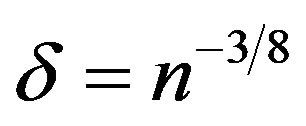 .
.
As  decreases in
 ,
,
 (23)
(23)
We will now show that  is dominated by a term of the form
 . Indeed, form C1), C2), 16) and 17) it follows that
 (24)
(24)
From which we get
 (25)
(25)
Thus, for  with
with  the integral
  is negligibly small. We now turn to the precise evaluation of the central integral
 . Since

we have
 (26)
(26)
We now unifiable proceed our proof for both conditions A) and B) and working analogously as in Kyriakoussis and Vamvakari [1] we get our final estimation (7).
In the previous theorem due to saddle point method principles, we have chosen the radius r of the derived asymptotic expansion (7) to be the solution of  . By solving this saddle point equation we get that

and

So, by substituting these to our estimation (7) the following corollary is proved.
Corollary 1. The q-factorial numbers of order  where A)

or B) 
have the following asymptotic expansion for 
 (27)
(27)
2.2. Deformed Gaussian Limiting Behaviour for the q(n)-Binomial Distributions with  as
as 
Transferred from the random variable X of the qbinomial distribution (1) to the equal-distributed deformed random variable , the mean value and variance of the random variable
 , say
, say  and
and  respectively, are given by the next relations
 (28)
(28)
and
 (29)
(29)
(see Kyriakoussis and Vamvakari [1]).
Using the standardized r.v.

with  and
and  given in (28) and (29), the
  -analogue Stirling asymptotic formula (27) and inspired by [1], the following theorem explores the continuous limiting behaviour of the
  -binomial distribution with
  as
as .
.
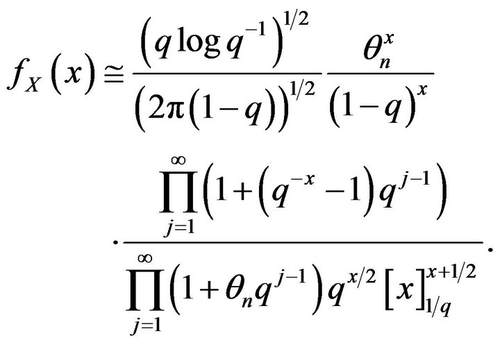
Theorem 2. Let the p.f. of the q-binomial distribution be of the form

where  such that
  as
as . Then, for A)
or B)

the  -binomial distribution is approximated, for
  by a deformed standardized Gauss distribution as follows
 (30)
(30)
Proof. Using the  -analogue of Stirling type (27), for
 with
with 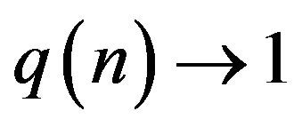 and
and  or
or
 , the
, the  -binomial distribution (1), is approximated by
 (31)
(31)
Let the random variable  and the qstandardized r.v.
  with
with  and
and 
given by (28) and (29) respectively, then all the following listed estimations are easily derived
 (32)
(32)
 (33)
(33)
 (34)
(34)
 (35)
(35)
Also, the estimation of the next product
 (36)
(36)
is derived by applying the Euler-Maclaurin summation formula (see Odlyzko [8], p. 1090) in the sum of the above Equation (36) as follows
 (37)
(37)
where  the dilogarithmic function and
  the Bernoulli number of order 2.
Moreover, working similarly for the sum appearing in the product
 (38)
(38)
the next estimation is obtained
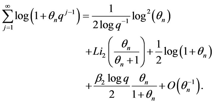 (39)
(39)
Applying all the previous the estimations (32)-(39) to the approximation (31), carrying out all the necessary manipulations and for , by both conditions A) and B), we derive our final asymptotic (30).
Remark 2. A realization of the sequence  considered in the above theorem 1A) is

with

Remark 3. Possible realizations of the sequence  considered in the above theorem 2B) are among others the next two ones

Corollary 2 Let the random variable  with p.f. that of the
  -binomial distribution as in Theorem 2. Then for
  the following approximation holds
 (40)
(40)
where
 (41)
(41)
with  the Gauss error function.
Proof. Using the approximation (2) and the classical continuity correction we have that
 (42)
(42)
Setting

the approximation (42) becomes
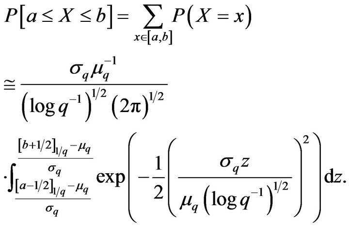 (43)
(43)
Carrying out all the necessary manipulations, we get the final approximation (40). 
3. Figures Using Maple
In this section, we present a computer realization of approximation (30), by providing figures using the computer program MAPLE and the  -series package developed by F. Garvan [13] which indicate good convergence even for moderate values of n. Analytically, for the random variable X, we give the Figures 1 and 2 realizing Theorem 2(A), by demonstrating with diamond blue points the exact probability
 (44)
(44)
and with diamond green points the continuous probability approximation
 (45)
(45)
with  and
and  given by Equation (41), for

and 
Note that similar good convergence even for moderate values of  have been implemented for Theorem 2B).
The procedure in MAPLE which realizes the exact probability (44) and its approximation (45) for given  and theta for both Theorem 2A) and 2B), is available under request.
4. Concluding Remarks
In this article, a deformed Gaussian limiting behaviour

Figure 1. Sketch of exact probability (44) by blue diamond points and probability approximation (45) by green diamond points, for n = 50.

Figure 2. Sketch of exact probability (44) by blue diamond points and probability approximation (45) by green diamond points, for n = 100.
for the  -Binomial distribution has been established. The proofs have been concentrated on the study of the sequence
  and the parameters of the considered distributions as sequences of
  Further, figures using the program MAPLE have been presented, indicating the accuracy of the established distribution convergence even for moderate values of n.
5. Acknowledgements
The author would like to thank Professor A. Kyriakoussis for his helpful comments and suggestions.