Nonconforming Mixed Finite Element Method for Nonlinear Hyperbolic Equations ()
1. Introduction
In this paper, we discuss a nonconforming mixed finite element method for the following nonlinear hyperbolic initial and boundary value problem.
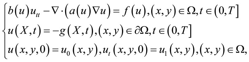 (1)
(1)
In order to describe the results briefly, we suppose that Equation (1) satisfy following assumptions on the data:
1)  and
and  are smooth and there exist constants
  and
and  satisfying
 .
.
2)  and
and  are sufficiently smooth functions with bounded derivatives.
There have been many very extensive studies about this kind of hyperbolic equations. For example, [1-3] studied the linear situations and gave error estimates under semi-discrete and fully-discrete schemes by standard Galerkin methods. [4,5] considered the mixed finite element methods for linear hyperbolic equations and obtained L2 prior estimates about continuous time. In addition, [6] analyzed the mixed finite element methods for second order nonlinear hyperbolic equations. But all the above investigations are mainly about conforming situations and projections are indispensable. As we know, the nonconforming finite element methods arise because of the demands for reducing the calculation cost. [7] has pointed that the nonconforming finite element methods with degree of freedom defined on the element edges or element itself are appropriate for each degree of freedom belong to at most elements.
In the present work, we focus on the nonconforming mixed finite element approximation scheme for nonlinear hyperbolic equations. Firstly, we introduce the corresponding space and the interpolation operators. Secondly, Existence and uniqueness of the solutions to the discrete problem are proved. Finally, Priori estimates of optimal order are derived for both the displacement and the stress.
Throughout this paper, C denotes a general positive constant which is independent of , and
, and  is the diameter of the finite element K.
2. Construction of the Elements
Let  be the a rectangular subdivision of
 and
and  satisfy the regular condition. For every K, let
  be the barycenter, the length of edges parallel to x-axis and y-axis by
  and
and . Then there exists an affine mapping
  where
where  is the reference element in
  plane and
  is the edges. We define the finite element
  on
on  as
as

 ,
,
 ,
,
 .
.
The interpolation functions defined above are properly and can be expressed as:
 ,
,

 ,
, . And For every
 , the associated finite element spaces as
 ,
,

where  denotes the jump of w across the boundary F, and
 , if
, if .
. 
 , the interpolation operators:
 .
.
 .
.
3. Main Results in Semi-Discrete Scheme
In this section, we will give the main results in this paper, including the existence and uniqueness of the solution to the discrete problem and priori estimates of optimal order.
Firstly, we introduce

and rewrite the Equation (1) as a system:

Secondly, for our subsequent use, we employ the classical Sobolev space  with norm
 . When
 , we simply write
  as
as . Furthermore, we denote the natural inner production in
  by
by  and the norm by
 , and let
 ,
,
 .
.
Thus the corresponding weak formulation of Equation (1) is to find a pair of , such that
 satisfying
 (2)
(2)
where .
.
The semi-discrete mixed finite element procedure is determined: , such that
 (3)
(3)
where . We define that
 ,
,
 .
.
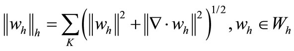
It can be seen that  and
and  are the norms for
  and
and , respectively.
Theorem 1. The above problem (3) has a unique solution.
Proof: Let  and
and  are bases of
  and
and , which satisfy

Then semi-discrete scheme can be rewritten as: Find  and
and , such that for every
  satisfy

here
 ,
,  ,
,
 ,
, 
 By the definition of the approximation spaces, we know that E is reversible and
 . Thus there holds that
 .
.
Since  and
and  are Lipschitz continuous, it has a unique solution according to the theory of differential equations [8].
Lemma 1. For 
 there hold that


Proof: Firstly, by the interpolation condition and definition, it is easy to see that  and
and
 . Secondly, for every
 , v is a constant, by application of Green’s formula and the interpolation definition yields that

Thus, we complete the proof of Lemma 1.
Lemma 2. [9] For , there hold that
 ,
, 
Now we give the main result of this paper.
Theorem 2. Let  and
and  be the solutions of Equations (2) and (3), respectively. For
  , there hold that

Proof: Let ,
, .
.
It is easy to see that  and
and  satisfy the following error equations
 (4)
(4)
and
 (5)
(5)
Using derivation about time t of Equation (4), combining Equation (5), we obtain
 (6)
(6)
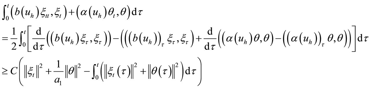
Choosing  and
and  in Equation (6), and integrating from 0 to t, we have
 (7)
(7)
We will give the analysis result of Equation (7) in detail. Firstly, by the initial condition, it is followed that
 (8)
(8)
Secondly, by Cauchy-Schwartz’s inequality and Young’s inequality, we obtain
 (9)
(9)
Similarly, by the initial condition of  and
and , we use Young’s inequality to get
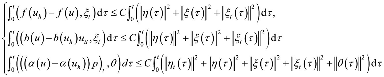 (10)
(10)
Substituting the above estimates, and applying Lemma 2, we get
 (11)
(11)
Then adding  at both sides Equation (11), and noticing that
 , we obtain that

Further, using Gronwall’s inequality to yield

By the interpolation theory (see [10]), we have
 .
.
Finally, by the triangle inequality, we complete the proof.