Hopf Bifurcation Analysis for a Modified Time-Delay Predator-Prey System with Harvesting ()
1. Introduction
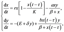
Due to its universal existence and importance, the study on the dynamics of predator-prey systems is one of the dominant subjects in ecology and mathematical ecology since Lotka [1] and Volterra [2] proposed the well- known predator-prey model [3]-[6]. Recently, a new method of central manifold has been developed to study the stability of delay induced bifurcation. In this paper, we study the following system:
 (1)
(1)
with
 (2)
(2)
where dot means differentiation with respect to time ,
,  and
and  are the prey and predator population densities, respectively. Parameter
  is the specific growth rate of prey in the absence of predation and without environment limitation.
  is environmental carrying capacity. The functional response of the predator is of Holling’s type with
 . And all parameters involved with the model are positive.
The purpose of this paper is to investigate the effect of time-delay on a modified predator-prey model with harvesting. We discussed the existence of Hopf bifurcation of system (1) and the direction of Hopf bifurcation and the stability of bifurcated periodic solutions are given.
2. Positive Equilibrium and Locally Asymptotically Stabiliy
After some calculations, we note system (1) has no boundary equilibria. However, it is more interesting to study the dynamical behaviors of the interior equilibrium points  and
and , where


The two distinct interior equilibrium points  exist whenever

holds.
We transform the interior equilibrium  to the origin by the transformation
 ,
, . Respectively, we still denote
 ![]() and
and ![]() by
by ![]() and
and![]() . Thus, system (1) is transformed into
. Thus, system (1) is transformed into
![]() (3)
(3)
First, we give the condition such that ![]() is locally stable. For simplicity, we denote
is locally stable. For simplicity, we denote
![]() (4)
(4)
The characteristic polynomial of ![]() is
is
![]() (5)
(5)
where
![]()
![]()
Now we consider the locally asymptotically stabiliy of the system without time-delay. Then we have
![]() (6)
(6)
If
![]()
holds, then it follows from the Routh-Hurwitz criterion that two roots of (6) have negative real parts.
Theorem 1. If ![]() and
and ![]() hold, the interior equilibrium point
hold, the interior equilibrium point ![]() of system (1) is locally asymptotically stable.
of system (1) is locally asymptotically stable.
3. Hopf Bifurcaion
In the section, we study whether there exists periodic solutions of system (1) about the interior equilibrium point![]() . Now we have the following results.
. Now we have the following results.
Theorem 2. If the system (1) satisfies the hypothesis ![]()
![]() and
and ![]() holds, then there exists a critical point
holds, then there exists a critical point ![]() such that the positive equilibrium point
such that the positive equilibrium point ![]() is locally asymptotically stable for
is locally asymptotically stable for ![]() and unstable for
and unstable for![]() , where
, where ![]() is defined in Equation (14).
is defined in Equation (14).
By the use of the instability result for the delayed differential Equations, in order to prove the instability of the equilibrium point, it is sufficient to show that there exists a purely imaginary ![]() and a positive real
and a positive real ![]() such that
such that
![]() (7)
(7)
where ![]() is defined in Equation (5).
is defined in Equation (5).
If ![]() is a root of Equation (7), then we have
is a root of Equation (7), then we have
![]() (8)
(8)
which leads to
![]() (9)
(9)
Let![]() , then Equation (9) takes the form
, then Equation (9) takes the form
![]() (10)
(10)
Since ![]() holds, we have
holds, we have![]() , which leads to
, which leads to![]() . Thus Equation (10) has at least one positive root, which leads to
. Thus Equation (10) has at least one positive root, which leads to
![]() (11)
(11)
Set ![]() as the root of Equation (8) with
as the root of Equation (8) with![]() , we have
, we have
![]() (12)
(12)
where
![]() (13)
(13)
Then ![]() are a pair of simple purely imaginary roots of Equation (8) with
are a pair of simple purely imaginary roots of Equation (8) with![]() , and we have
, and we have
![]() (14)
(14)
Then by the Butler’s Lemma, ![]() is unstable for
is unstable for![]() . On the other hand, if
. On the other hand, if![]() , then Equation (7) have no roots on the imaginary axis. Then Equation (7) for
, then Equation (7) have no roots on the imaginary axis. Then Equation (7) for![]() , only has negative real part roots, which implies that
, only has negative real part roots, which implies that ![]() is locally asymptotically stable for
is locally asymptotically stable for![]() .
.
Theorem 3. If the system (1) satisfies the hypothesis ![]()
![]() and
and![]() , then the system (1) undergoes Hopf bifurcation at
, then the system (1) undergoes Hopf bifurcation at ![]() when
when![]() .
.
Proof. The Hopf bifurcation will be proved if we can show that
![]() (15)
(15)
From Equation (7), we have
![]() (16)
(16)
Substituting Equation (8) into Equation (16), we have
![]() (17)
(17)
Substituting Equation (14) into the above equation, we have
![]()
Therefore, the transversality condition is satisfied. Therefore Hopf bifurcation occurs at![]() .
.
4. The Direction and Stability of the Hopf Bifurcation
In this section, we analyze the direction and stability of the Hopf bifurcation of (3) obtained in Theorem 3 by taking ![]() as the bifurcation parameter.
as the bifurcation parameter.
Let![]() , then
, then ![]() is the Hopf bifurcation value of system (3). Rescale the time by
is the Hopf bifurcation value of system (3). Rescale the time by ![]() to normalize the delay. The periodic solution of system (3) is equivalent to the solution of the following system
to normalize the delay. The periodic solution of system (3) is equivalent to the solution of the following system
![]() (18)
(18)
We define ![]() as nonnegative integer, define
as nonnegative integer, define ![]() as follows
as follows
![]()
Rewrite system (18) to
![]() (19)
(19)
where
![]() (20)
(20)
We use the method which is based on the center manifold and normal form theory, and define![]() . Then the system (19) is transformed into a functional differential equation as
. Then the system (19) is transformed into a functional differential equation as
![]() (21)
(21)
where ![]() and
and ![]() are respectively represented by
are respectively represented by
![]() (22)
(22)
and
![]() (23)
(23)
where![]() . By the Riesz representation theorem, there exist a
. By the Riesz representation theorem, there exist a ![]() matrix
matrix![]() , whose elements are of bounded variation functions such that
, whose elements are of bounded variation functions such that
![]() (24)
(24)
In fact, we can choose
![]() (25)
(25)
where ![]() is the Dirac delta function. For
is the Dirac delta function. For![]() , we define
, we define
![]() (26)
(26)
and
![]() (27)
(27)
Thus system (21) is equivalent to
![]() (28)
(28)
where ![]() for
for![]() .
.
For![]() , define
, define
![]() (29)
(29)
and a bilinear inner product
![]() (30)
(30)
where![]() . Then
. Then ![]() and
and ![]() are adjoint operators. From the discussion in Theorem 2, we know that
are adjoint operators. From the discussion in Theorem 2, we know that ![]() are eigenvalues of
are eigenvalues of ![]() and therefore they are also eigenvalues of
and therefore they are also eigenvalues of![]() .
.
Suppose ![]() is the eigenvector of
is the eigenvector of ![]() corresponding to
corresponding to![]() . Thus,
. Thus,![]()
![]() . From the definition of
. From the definition of ![]() we have
we have
![]()
Then we have
![]() (31)
(31)
Similarly, let ![]() be the eigenvector of
be the eigenvector of ![]() corresponding to
corresponding to![]() . Then by
. Then by ![]() and the definition of
and the definition of![]() , we obtain
, we obtain
![]()
Therefore
![]() (32)
(32)
In order to ensure, we need to determine the value of![]() , from Equation (29) we have
, from Equation (29) we have
![]() (33)
(33)
Then we can choose ![]() such as
such as
![]() (34)
(34)
where ![]() is the conjugate complex number of
is the conjugate complex number of![]() .
.
Next we will compute the coordinate to describe the center manifold ![]() at
at![]() . Let
. Let ![]() be the solution of Equation (27) when
be the solution of Equation (27) when![]() . Define
. Define
![]() (35)
(35)
On the center manifold![]() , we have
, we have![]() , where
, where
![]() (36)
(36)
![]() and
and ![]() are local coordinates for the center manifold
are local coordinates for the center manifold ![]() in the direction of
in the direction of ![]() and
and![]() . Note that
. Note that ![]() is real if
is real if ![]() is real. We only concern with the real solutions. For solution
is real. We only concern with the real solutions. For solution ![]() of Equation (27), since
of Equation (27), since ![]() and Equation (35), we have
and Equation (35), we have
![]() (37)
(37)
We rewrite above equation as
![]() (38)
(38)
where
![]() (39)
(39)
From Equation (35) and Equation (36), we obtain that
![]() (40)
(40)
Substituting Equation (23) and Equation (40) into Equation (39), we have
![]() (41)
(41)
where ![]() stands for higher order terms, and
stands for higher order terms, and
![]()
![]()
Comparing Equation (39) and Equation (41), we get
![]() (42)
(42)
Since ![]() depends on
depends on ![]() and
and![]() , we need to find the values of
, we need to find the values of ![]() and
and![]() . From Equation (21) and Equation (35), we have
. From Equation (21) and Equation (35), we have
![]() (43)
(43)
where
![]() (44)
(44)
From Equation (36), we have
![]() (45)
(45)
It follows from Equation (39) that
![]() (46)
(46)
Comparing the coefficients of ![]() and
and ![]() from Equation (45) and Equation (46), we get
from Equation (45) and Equation (46), we get
![]() (47)
(47)
Then for![]() , we have
, we have
![]() (48)
(48)
Comparing the coefficients of ![]() and
and ![]() between Equation (44) and Equation (48), we get
between Equation (44) and Equation (48), we get
![]() (49)
(49)
From the definition of ![]() and Equation (49), we have
and Equation (49), we have
![]() (50)
(50)
Since![]() , we obtain
, we obtain
![]() (51)
(51)
where ![]() is a constant vector. Similarly, we have
is a constant vector. Similarly, we have
![]() (52)
(52)
where ![]() is a constant vector. Now, we shall find the values of
is a constant vector. Now, we shall find the values of ![]() and
and![]() . From the definition of
. From the definition of ![]() and Equation (50), we have
and Equation (50), we have
![]() (53)
(53)
and
![]() (54)
(54)
where![]() . In view of Equation (43), we induce that when
. In view of Equation (43), we induce that when![]() .
.
![]() (55)
(55)
Then we have
![]() (56)
(56)
Comparing both sides of Equation (56), we obtain
![]() (57)
(57)
where ![]() and
and ![]() are respectively the coefficients of
are respectively the coefficients of ![]() and
and ![]() of
of![]() . Thus we have
. Thus we have
![]() (58)
(58)
where![]() .
.
Since ![]() is the eigenvalue of
is the eigenvalue of ![]() and
and ![]() is the corresponding eigenvector, we get
is the corresponding eigenvector, we get
![]() (59)
(59)
![]() (60)
(60)
Therefore, substituting Equation (53) and Equation (59) into Equation (60), we have
![]() (61)
(61)
that is
![]() (62)
(62)
where
![]() (63)
(63)
Thus![]() ,
, ![]() , and
, and ![]() is the value of the determinant
is the value of the determinant![]() , where
, where ![]() is formed by replacing the
is formed by replacing the ![]() th column vector of
th column vector of ![]() by another column vector
by another column vector ![]() for
for![]() . In a similar way, we have
. In a similar way, we have
![]() (64)
(64)
where
![]() (65)
(65)
Thus![]() , where
, where ![]() and
and ![]() is the value of the determinant
is the value of the determinant ![]() that is formed by replacing the
that is formed by replacing the ![]() th column vector of
th column vector of ![]() by another column vector
by another column vector ![]() for
for![]() . Therefore, we can determine
. Therefore, we can determine ![]() and
and ![]() from Equation (51) and Equation (52). Furthermore, we can easily compute
from Equation (51) and Equation (52). Furthermore, we can easily compute![]() .
.
Then the Hopf bifurcating periodic solutions of system (1) at ![]() on the center manifold are determined by the following formulas
on the center manifold are determined by the following formulas
![]() (66)
(66)
Here ![]() determines the direction of Hopf bifurcation. If
determines the direction of Hopf bifurcation. If![]() , then the Hopf-bifurcation is forward(backward) and the bifurcating periodic solutions exist for
, then the Hopf-bifurcation is forward(backward) and the bifurcating periodic solutions exist for![]() . Again
. Again ![]() determines the stability of the bifurcating periodic solutions. The bifurcating periodic solutions are stable (unstable) if
determines the stability of the bifurcating periodic solutions. The bifurcating periodic solutions are stable (unstable) if![]() .
. ![]() determines the period of periodic solutions: the period increases (decreases) if
determines the period of periodic solutions: the period increases (decreases) if![]() . Therefore, we have the following results.
. Therefore, we have the following results.
Theorem 4. The Hopf bifurcation of the system (1) occurring at ![]() when
when ![]() is forward (backward) if
is forward (backward) if ![]() and the bifurcating periodic solutions on the center manifold are stable (unstable) if
and the bifurcating periodic solutions on the center manifold are stable (unstable) if ![]() .
.
5. Conclusion
This paper introduces modified time-delay predator- prey model. Then we study the Hopf bifurcation and the stability of the system. Our results reveal the conditions on the parameters so that the periodic solutions exist surrounding the interior equilibrium point. It shows that ![]() is a critical value for the time delay
is a critical value for the time delay![]() . Furthermore, the direction of Hopf bifurcation and the stability of bifurcated periodic solutions are investigated.
. Furthermore, the direction of Hopf bifurcation and the stability of bifurcated periodic solutions are investigated.
Acknowledgements
This project is jointly supported by the National Natural Science Foundations of China (Grant No. 61074192). We also would like to thank the anonymous referees which have improved the quality of our study.