Existence of Solutions to Path-Dependent Kinetic Equations and Related Forward-Backward Systems ()
1. Introduction
For a Banach space B we denote by B* the dual Banach space of B. The pairing between  and
and  is denoted by
 . The norm in B* is defined by
 . For a
 , we denote by
 the Banach space of continuous curves
  equipped with the norm
 .
.
A deterministic dynamic in  can be naturally specified by a vector-valued ordinary differential equation
 (1)
(1)
with a given initial value , where the mapping
  is from
  to
to . More generally, one often meets the situations when
  does not belong to
 , but to some its extension. Namely, let
  be a dense subset of
 , which is itself a Banach space with the norm
 . A deterministic dynamic in
  can be specified by Equation (1), where the mapping
  is from
  to
to . Written in weak form, Equation (1) means that, for all
 ,
,
 (2)
(2)
In many applications, Equation (2) appears in the form
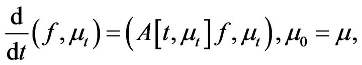 (3)
(3)
where the mapping  is from
  to bounded linear operators
  such that, for each pair
 ,
,  generates a strongly continuous semigroup in
 . Of major interest is the case when
  is the space of measures on a locally compact space. It turns out that, in this case and under mild technical assumptions, an evolution (2) preserving positivity has to be of form (3) with the operators
  generating Feller processes, see Theorems 6.8.1 and 11.5.1 from [1].
Equation (3) contains most of the basic equations from non-equilibrium statistical mechanics and evolutionary biology, see monograph [1] for an extensive discussion.
In this paper we are mostly interested in yet more general equation. Namely, let  be a closed convex subset of
 , which is also closed in
 . For a
 , let
, let  denote a closed convex subset of
 consisting of curves with values in
 , and
, and  a closed convex subset of
 , consisting of curves
  with initial data
 .
.
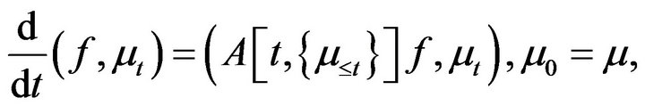
The main object of this paper is a “path-dependent” version of Equation (3), that is
 (4)
(4)
where

maps  to bounded linear operators
 . We refer to equation (4) as the general path-dependent kinetic equation. It should hold for all test functions
 . Compared to Equation (4), Equation (3) is often referred to as a path-independent case.
When the operators  only depend on the history of the trajectory of
 , that is
 (5)
(5)
we call (5) an adapted kinetic equation, where  is a shorthand for
 . Adapted kinetic equations can be seen as analytic analogs of stochastic differential equations with adapted coefficients, and their well-posedness can be obtained by similar methods. When the generators
  only depend on the future of the trajectory of
 , that is
 (6)
(6)
we call (6) an anticipating kinetic equation, where  is a shorthand for
 .
.
Equation (1.4) has many applications. Let us briefly explain the crucial role played by this equation in the mean field game (MFG) methodology, which is based on the analysis of coupled systems of forward-backward evolutions and which constitutes a quickly developing area of research in modern theory of optimization, see detail e.g. in [2-4].
Assume that the objective of an agent described by a controlled stochastic process  (passing through x at time t), given an evolution
  of the empirical distributions of a large number of other players, is to maximize (over a suitable class of controls
 ) the payoff

By dynamic programming the optimal payoff  of such an agent, which equals
 should satisfy certain HJB equation (backward evolution). On the other hand, when all optimal controls
  are found, the empirical measure
  of the resulting process satisfies the controlled kinetic equation of type (3) (forward equation), that is
 (7)
(7)
The main consistency condition of MFG is in the requirement that the initial  coincides with the resulting
 . Equalizing
  in (7) clearly leads to anticipating kinetic equation of type (6).
Our main results concern the well-posedness of adaptive kinetic Equations (5), the local well-posedness and global existence of anticipating and general path dependent kinetic equations and finally some regularity result for path-independent equations arising from their probabilistic interpretations. This yield an improved version of the existence results of the unpublished preprint [4].
2. Main Results
Let us recall the notion of propagators needed for the proper formulation of our results.
For a set S, a family of mappings  from S to itself, parametrized by the pairs of numbers
  (resp.
 ) from a given finite or infinite interval is called a (forward) propagator (resp. a backward propagator) in S, if
  is the identity operator in S for all t and the following chain rule, or propagator equation, holds for
  (resp. for
 ):
):

A backward propagator  of bounded linear operators on a Banach space B is called strongly continuous if the operators
  depend strongly continuously on t and r.
Suppose  is a strongly continuous backward propagator of bounded linear operators on a Banach space with a common invariant domain
 . Let
. Let , be a family of bounded linear operators
  that are strongly continuous in
  outside a set
  of zero-measure in
 . Let us say that the family
  generates
  on
on  if, for any
 , the equations
 (8)
(8)
hold for all s outside S with the derivatives taken in the topology of B. In particular, if the operators  depend strongly continuously on
 , equations (8) hold for all s and
 , where for
  (resp.
 ) it is assumed to be only a right (resp. left) derivative. In the case of propagators in the space of measures, the second equation in (8) is called the backward Kolomogorov equation.
We can now formulate our main results.
Theorem 2.1 (local well-posedness for general “pathdependent” case) Let  be a bounded convex subset of
  with
with , which is closed in the norm topologies of both
  and
and . Suppose that 1) the linear operators
  are uniformly bounded and Lipschitz in
 , i.e. for any
 (9)
(9)
 (10)
(10)
for a positive constant ;
;
2) for any , let the operator curve
  generate a strongly continuous backward propagator of bounded linear operators
  in
in ,
,  , on the common invariant domain
 , such that
 (11)
(11)
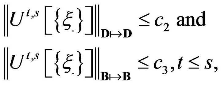
for some positive constants , and with their dual propagators
  preserving the set
 .
.
Then, if
 (12)
(12)
the Cauchy problem (4) is well posed, that is for any , it has a unique solution
  (that is (4) holds for all
 ) that depends Lipschitz continuously on time t and the initial data in the norm of
 , i.e.
 (13)
(13)
and for 
 (14)
(14)
Theorem 2.2 (global wellposedness for an “adapted” case) Under the assumptions in Theorem 2.1, but without the locality constraint (12), the Cauchy problem (5) is well posed in  and its unique solution depends Lipschitz continuously on initial data in the norm of
 .
.
Theorem 2.3 (global existence of the solution for general “path dependent”case) Under the assumptions in Theorem 2.1, but without the locality constraint (12), assume additionally that for any  from a dense subset of
 , the set
 (15)
(15)
is relatively compact in . Then a solution to the Cauchy problem (4) exists in
 .
.
In Proposition 4.3 in Section 4, we give the conditions under which the compactness assumption (15) holds.
3. Proofs of the Main Results
Proof of Theorem 2.1
By duality, for any 

By (8),

Then, together with assumptions (9) and (11),
 (16)
(16)
Consequently, if (12) holds, the mapping
 is a contraction in
 . Hence by the contraction principle there exists a unique fixed point for this mapping and hence a unique solution to Equation (4).
Inequality (13) follows directly from (4). Finally, if  and
and , then

From (11) and (16),
 (17)
(17)
implying (14).
Proof of Theorem 2.2
For a , let us construct an approximating sequence
 , by defining
  for
for  and then recursively
 . By non-anticipation, arguing as in the proof of (16) above, we first get the estimate
 and then recursively
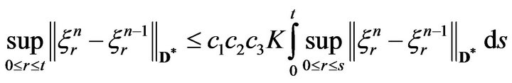
that implies (by straightforward induction) that, for all ,
,

Hence, the partial sums on the r.h.s. of the obvious equation

converge, and thus the sequence  converges in
  . The limit is clearly a solution to (5).
Finally, let us assume that  and
and  are some solutions with the initial conditions
  and
and  respectively. Instead of (17), we now get

By Gronwall’s lemma, this implies that
 does not exceed
 yielding uniqueness and Lipchitz continuity of solutions with respect to initial data.
Proof of Theorem 2.3
Since  is convex, the space
is also convex. Since the dual operators  preserve the set
 , for any
 the curve
  belongs to
  as a function of
 . Hence, the mapping

is from  to itself. Moreover, by (16), this mapping is Lipschitz continuous.
Denote
 .
.
Together with (13), the assumption that set (15) is compact in  for any
  from a dense subset of
  implies that the set
  is relatively compact in
 (by the Arzela-Ascoli Theorem).
Finally, by Schauder fixed point theorem, there exists a fixed point in , which gives the existence of a solution to (4).
4. Nonlinear Markov Evolutions and Its Regularity
This section is designed to provide a probabilistic interpretation and, as a consequence, certain regularity properties for nonlinear Markov evolution  solving kinetic Equation (3) in the case when
  is the Banach space of bounded continuous functions f on
  with
with , equipped with sup-norm and
  is the set of probability measures on
 , so that
  is the space of signed Borel measures on
 and
and . As a consequencewe shall present a simple criterion for the main compactness assumption of Theorem 2.3.
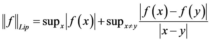
We shall denote  the Banach space of bounded Lipschitz continuous functions f on
  with the norm
and  (resp.
 ) the Banach space of continuously differentiable functions f on
  such that f and the derivative
  belongs to
 , equipped with the norm

resp. twice continuously differentiable with 
 and the norm
 .
.
Let  be a family of operators in
  of the Lévy-Khintchin type, that is
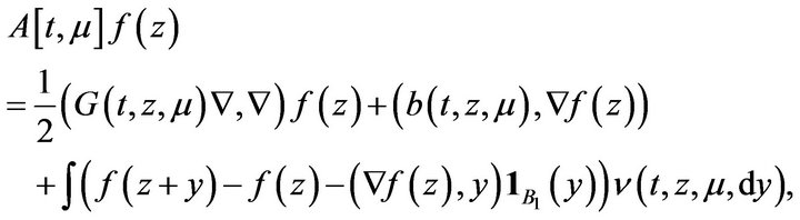 (18)
(18)
where  denotes the gradient operator; for
  ,
,  is a symmetric non-negative matrix,
  is a vector,
  is a Lévy measure on
 , i.e.
 (19)
(19)
depending measurably on , and
, and  denotes, as usual, the indicator function of the unit ball in
 . Assume that each operator (18) generates a Feller process with one and the same domain
  such that
  .
.
Proposition 4.1 Suppose the assumptions of Theorem 2.2 are fulfilled with generators  of “path-independent” type (3) and a probability measure
  is given. Then there exists a family of processes
  defined on a certain filtered probability space
  such that
  solves the Cauchy problem for Equation (3) with initial condition
  and
and  solves the nonlinear martingale problem, specified by the family
 , that is, for any
 ,
,
 (20)
(20)
is a martingale.
By the assumptions of Theorem 2.2, a solution  of Equation (3) with initial condition
  specifies a propagator
 , of linear transformations in
 , solving the Cauchy problems for equation
 (21)
(21)
In its turn, for any , Equation (21) specifies marginal distributions of a usual (linear) Markov process
  in
in  with the initial measure
 . Clearly, the process
  is a solution to our martingale problem.
We shall refer to the family of processes constructed in Proposition 4.1 as to nonlinear Markov process generated by the family .
.
Using martingales allows us to prove the following useful regularity property for the solution of kinetic equations.
Proposition 4.2 Suppose the assumptions of Theorem 2.2 are fulfilled for a kinetic equation of “path-independent” type (3) with generators  of type (18). Let
  denote a nonlinear Markov process constructed from the family of generators
  by Proposition 4.1. Assume, for
  and
and , the following boundedness condition holds:
 (22)
(22)
and  for the initial measure
 .
.
Then the distributions , solving the Cauchy problem for Equation (3) with initial condition
  have uniformly bounded pth moments, i.e.
 (23)
(23)
and are  -Hölder continuous with respect to t in the space
 , i.e.
 (24)
(24)
with a positive constant .
.
Proof. For a fixed trajectory  with initial value
 , one can consider
  as a usual Markov process. Using the estimates for the moments of such processes from formula (5.61) of [5] (more precisely, its straightforward extension to time non-homogeneous case), one obtains from (22) that
 (25)
(25)
This implies (23) and the estimate
 (26)
(26)
where constants  can have different values in various formulas above.
Since  is the distribution law of the process
 ,
,
 (27)
(27)
From (26), (27) and Markov property, we get (24) as required.
Remark 4.1 For diffusions with , (24) was proved in [3].
Our main purpose for presenting Proposition 4.2 lies in the following corollary that follows from (23) and an observation that a set of probability laws on  with a bounded
  th moment,
  , is tight.
Proposition 4.3 Under the assumptions of Theorem 2.1 for generators  of Lévy-Khintchin type (18), but without locality condition (12), suppose the boundedness condition (22) holds for some
  and
and . Then the compactness condition from Theorem 2.3 (stating that set (15) is compact in
 ) holds for any initial measure
  with a finite moment of
  th order.
5. Basic Examples of Operators 
We present here basic examples of generators that fit to our main Theorems and are relevant to the study of mean field games. The most nontrivial condition of Theorem 2.1 is 2).
The simplest examples are McKean-Vlasov diffusions defined by SDE

with corresponding generator

where the condition of Theorem 2.1 2) is known to follow, for Lipshitz continuous coefficients, from Ito’s calculus.
Another example is supplied by nonlinear Lévy processes that are specified by generators of type (18) such that all coefficients do not depend on z, i.e.

It follows from Proposition 7.1 of [1] that if the coefficients  are continuous in t and Lipschitz continuous in
  in the norm of Banach space
 , i.e.

with a positive constant c, then condition 2) of Theorem 2.1 holds with . Notice also that the usual examples of a functional F on measures given by monomials
  are Lipschitz continuous (or even smooth) in space
  whenever g is sufficient smooth.
Another example is supplied by processes (describing lots of models including spatially homogeneous and mollified Boltzmann equation and interacting  -stable laws with
 ) with generators of order at most one

with the Lévy measures  having finite first moment
 . As is established in Theorem 4.17 of [1], if
  are continuous in t, Lipshitz continuous in
  and Lipschitz continuous in
 , that is,
  ,
,  ,
,

then condition 2) of Theorem 2.1 is satisfied with  .
.
As other examples let us mention pure jump processes with bounded rates, where the conditions of Theorem 2.1 are satisfied with , and nonlinear stablelike processes (see [1]).
Let us note finally that not all interesting evolution of type (3) satisfy our Lipschitz continuity assumption. A different type of continuity should be applied for coefficients depending on measures via quantiles, e.g. value at risk (VAR), which is analyzed in [6] inspired by preprint [7].
NOTES