Mapping Properties of Generalized Robertson Functions under Certain Integral Operators ()
1. Introduction
Let  be the class of functions
  of the form

which are analytic in the open unit disc . We write
 . A function
  is said to be spiral-like if there exists a real number

such that

The class of all spiral-like functions was introduced by L. Spacek [1] in 1933 and we denote it by . Later in 1969, Robertson [2] considered the class
  of analytic functions in
  for which
 .
.
Let  be the class of functions
  analytic in
  with
with  and
and

where ,
,  and
and  is real with
 .
.
For ,
,  , this class was introduced in [3] and for
 , see [4]. For
 ,
,  and
and , the class
  reduces to the class
  of functions
  analytic in
  with
with  and whose real part is positive.
We define the following classes


For ,
,  and
and , we obtain the well known classes
  and
and  of analytic functions with bounded radius and bounded boundary rotations studied by Tammi [5] and Paatero [6] respectively. For details see [7-12]. Also it can easily be seen that
  and
and 
Let us consider the integral operators
 (1.1)
(1.1)
and
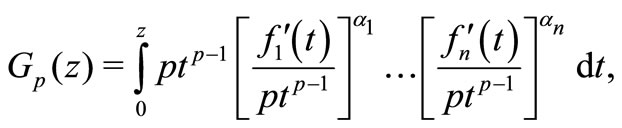 (1.2)
(1.2)
where  and
and  for all
  .
.
These operators, given by (1.1) and (1.2), are defined by Frasin [13]. If we take , we obtain the integral operators
  and
and  introduced and studied by Breaz and Breaz [14] and Breaz et al. [15], for details see also [16-20]. Also for
 ,
,  in (1.1), we obtain the integral operator studied in [21] given as

and for ,
,  ,
,  in (1.2), we obtain the integral operator

discussed in [22,23].
In this paper, we investigate some propeties of the above integral operators  and
and  for the classes
  and
and respectively.
2. Main Result
Theorem 2.1. Let  for
for  with
with
 . Also let
  is real with
 ,
,  ,
,
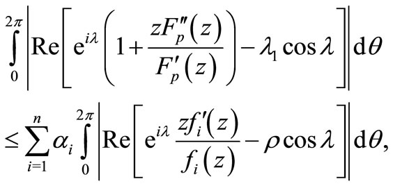
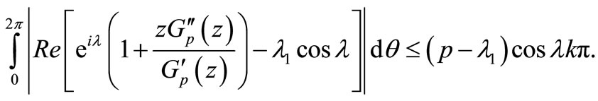
 . If
. If

then  with
with
 (2.1)
(2.1)
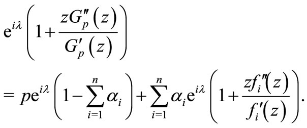
Proof. From (1.1), we have
 (2.2)
(2.2)
or, equivalently
 (2.3)
(2.3)
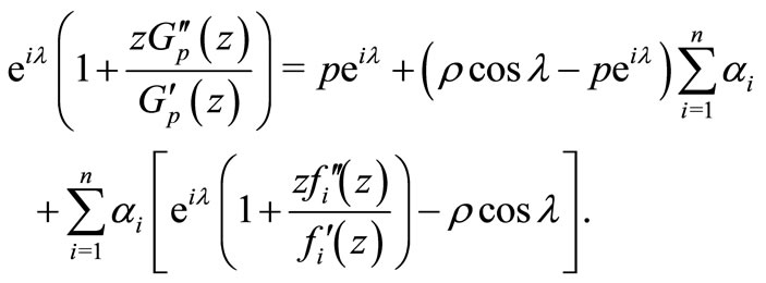
Subtracting and adding  on the right hand side of (2.3), we have
 (2.4)
(2.4)
Taking real part of (2.4) and then simple computation gives
 (2.5)
(2.5)
where  is given by (2.1). Since
  for
for , we have
 (2.6)
(2.6)
Using (2.6) and (2.1) in (2.5), we obtain
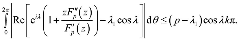
Hence  with
with  is given by (2.1).
By setting  and
and  in Theorem 2.1, we obtain the following result proved in [9].
Corollory 2.2. Let  for
for  with
with . Also let
 ,
, . If
. If

then  and
and  is given by (2.1).
Now if we take  and
and  in Theorem 2.1, we obtain the following result.
Corollory 2.3. Let  for
for  with
with . Also let
 ,
, . If
. If

then  and
and  is given by (2.1).
Letting ,
,  ,
,  and
and  in Theorem 2.1, we have.
Corollory 2.4. Let  with
with . Also let
 . If
. If

then

with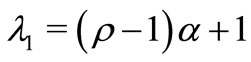 .
.
Theorem 2.5. Let  for
for 
with . Also let
  is real is real with
 ,
,
 ,
, . If
. If

then  and
and  is given by (2.1).
Proof. From (1.2), we have

or, equivalently
This relation is equivalent to
 (2.7)
(2.7)
Taking real part of (2.7) and then simple computation gives us
 (2.8)
(2.8)
where  is given by (2.1). Since
  for
for , we have
 (2.9)
(2.9)
Using (2.9) in (2.8), we obtain
Hence 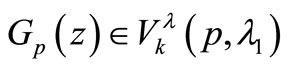 with
with  is given by (2.1).
By setting  and
and  in Theorem 2.5, we obtain the following result.
Corollory 2.6. Let  for
for  with
with . Also let
 ,
, . If
. If

then  with
with  is given by (2.1).
Letting ,
,  ,
,  and
and  in Theorem 2.5, we have.
Corollory 2.7. Let  with
with . Also let
 . If
. If , then
with .
.
NOTES