Dynamics Behaviors of a Reaction-Diffusion Predator-Prey System with Beddington-DeAngelis Functional Response and Delay ()
1. Introduction
Recently, the dynamics of predator-prey systems is one of the fastest developing areas of modern mathematics due to their significant nature in biological fields and other practical fields. One significant component in these systems is the functional response describing the number of prey consumed per predator per unit time for given quantities of prey N and predators P. The traditional mathematical model describing the predator-prey interactions consists of the following system of differential equations.
In recent years, many authors have explored the dynamic relationship between predators and their preys. There is extensive literature related to these topics for ordinary differential equation models (see [1] -[6] and the references cited therein). We know that more realistic prey-predator models were introduced by Holling suggesting three kinds of functional responses for different species to model the phenomena of predation [3] . On the other hand, species have the natural tendency to move from areas of bigger population concentration to those of smaller population concentration. This kind of diffusion process is called free diffusion and it is not considered in the above mentioned references. In the literature, many researchers have directly introduced the free diffusion to ODEs and DDEs and have also explained why to do so. To name a few, see [7] -[14] . Moreover, such models or similar models with delays and free diffusion have also arisen from a variety of situations like infectious disease dynamics, porous medium, chemical reaction, engineering control theory. Taking into account the inhomogeneous distribution of the species in different spatial locations within a fixed bounded domain , Peng and Wang looked at a diffusive HollingTanner prey-predator model in [7]
 (1.1)
(1.1)
where  and
and  represent the species densities of the prey and predator, respectively.
  is the outward unit normal vector on the smooth boundary
 .The constants
  are the diffusion coefficients corresponding to
  and
and , respectively, and all the parameters appearing in (1.1) are assumed to be positive. The admissible initial data
  and
and  are continuous functions on
 . The homogeneous Neumann boundary condition means that (1.1) is self-contained and has no population flux across the boundary
 . For more detailed biological implications of the model, one may further refer to [7] and the references cited therein.
In recent years, great attention has been paid to the study of the existence of traveling wave solutions in reactiondiffusion system, since they determine the long term behavior of other solutions, and account for phase transitions between different states of physical systems, propagation of patterns, and domain invasion of species in population biology (see, for example, [10] -[12] , and the references cited therein).
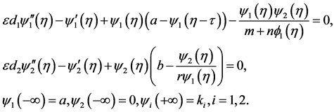
Motivated by the work of Peng and Wang [7] and Wu, Zou [12] , in the present paper, we consider the existence of traveling waves of the following predator-prey model with Beddington-DeAngelis functional response and a discrete time delay due to gestation of predator
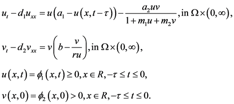 (1.2)
(1.2)
The main purpose of the paper is to consider the existence of traveling wavefronts for the delay model (1.2). In order to study traveling wavefronts, we need to analyze the stability of the positive constant equilibrium first. As a result, the remaining part of this paper is organized as follows. We first use linearized method to study the stability of the positive constant equilibrium of (1.2) in Section 2. Then, applying the method of upper and lower solutions, we establish the existence of traveling wavefronts of (1.2) in Section 3. At the same time, we give some suitable examples to illustrate our results.
2. Asymptotical Stability of the Positive
Constant Equilibrium
Set the right side of the system (1.2) to zero. It is easy to check that the system (1.2) has an axial equilibrium  and a unique positive equilibrium
 , where

And . In this section, we discuss the locally asymptotical stability of the positive constant equilibrium by the linearized method. The linearized system of (1.2) about a positive constant equilibrium
  is
is
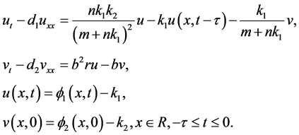 (2.1)
(2.1)
System (2.1) admits nontrivial solutions of the form  if and only if the determinant

which implies that
 (2.2)
(2.2)
where  is a complex number and
  is a real number (see, for example, Ge and He [11] and the references therein).
It is easy to check that , so, we rewrite (2.2) as
 (2.3)
(2.3)
We claim that , if
, if  satisfies (2.3) and
  is sufficiently small. Otherwise, suppose that there exists a
  satisfying (2.3) such that
 . Then direct computation gives us

We can prove that  So, if
  is sufficiently small, we have

It is a contradiction. This proves the claim. As a result, we have proved.
Theorem 2.1. The positive equilibrium  of (1.2) is locally asymptotically stable for
  sufficiently small.
Remark 2.1. In [7] , it was showed the following result: Suppose that . Then positive equilibrium of (1.1) is asymptotically stable. However, in this paper, we also obtain the asymptotical stability about the positive equilibrium without conditions in absence time delay
 .
.
In order to illustrate the validity of the theoretical result on the asymptotical stability, we perform numerical calculations using the software MATLAB.
Consider the following system:
the positive equilibrium  of system (1.2) is locally asymptotically stable (see Figure 1 and Figure 2).
3. Existence of Traveling Wavefront
A traveling wave solution of (1.2) is a special translation invariant solution of the from
 with wave speed c. Various methods including the monotone itera-
tion technique [11] [12] and the degree theory [10] have been adopted to study the existence of traveling wave solutions to reaction-diffusion systems with delays. In this section, we use the approach introduced by Canosa [14] to establish the existence of traveling wave solutions connecting the axial equilibrium  to the positive equilibrium
 . To seek such a pair of traveling wavefronts of (1.2), we substitute
  and
and , where
 , into (1.2) to obtain
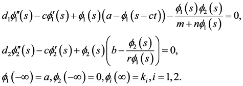 (3.1)
(3.1)
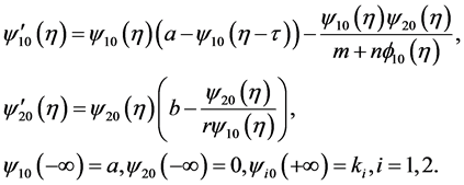
Now, we follow the approach of Canosa [14] to construct a uniformly valid asymptotic approximation to the wavefronts for large values of the wave speed c. Suppose that c is large enough. Then  is a small parameter. We aim to seek a pair of solutions to (3.1) of the form

Then (3.1) becomes
 (3.2)
(3.2)
Denote

and substitute them into (3.2). It turns out that  and
and  satisfy
 (3.3)
(3.3)
For simplicity of notation, we still denote 
 by
by , respectively. Then (3.3) becomes
 (3.4)
(3.4)
Now, we are ready to state and prove the following result by the upper and lower solution technique developed by Wu and Zou [12] .
Theorem 3.1. System (1.2) has a traveling wavefront connecting  to
to  for
for  sufficiently small.
Proof. The proof is divided into the following two steps.
Step I: Verify a quasi-monotonicity condition. For this purpose, we define the functional

by
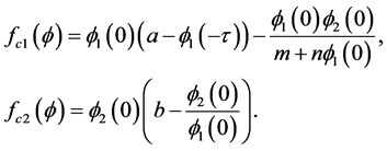 (3.5)
(3.5)
For arbitrary  and
and  such that

and  and
and  we have
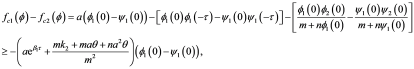
which implies

Similarly, we can get

Therefore, if we choose 
 , then by continuity we know that, for
  sufficiently small,
 . This proves the quasi-monotonicity condition.
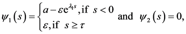
Step II: Establish the existence of a pair of upper and lower solutions. To achieve this, we look for wave front solutions of (3.1) in the following profile set


Define

And  where
where 
Then  We distinguish two cases to show that
  is a pair of upper solutions to (3.4).
Case I: s < 0. It is easy to see that

Thus

Similarly,

Case II: . We have

which implies that

Therefore,

and

The above discussion tells us that  is an upper solution to (3.4).
Now, define
 (3.6)
(3.6)
where
 (3.7)
(3.7)
Using (3.6)-(3.7) we have

if  and
and

if  This proves that
  is a pair of lower solutions to (3.4).
So far, we have verified all the assumptions in the theory developed by Wu and Zou [12] . Therefore, there exists at least one solution in the set , that is, system (1.2) has a traveling wavefront solution connecting
  to
to .This completes the proof.
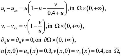
Remark 3.1. We study the existence of traveling wave for a reaction-diffusion Holling-Tanner model with delay. In order to illustrate the validity of the theoretical result obtained in this section, we also perform numerical calculations using the software MATLAB.
Consider the following Holling-Tanner system:
 (3.8)
(3.8)
It should satisfy the following boundary conditions:

where 
 Fix
Fix 
 Then system (3.8) has a positive equilibrium
 . By Theorem 3.1, we see that system (3.8) has a traveling wave solution connecting the axial solution
  with the positive equilibrium
  when the wave speed c is larger. Numerical simulation can be carried out by using MATLAB7.01. See Figure 3. However, when the wave speed c is smaller, the system (3.8) doesn’t exist the traveling wave solution. Following we also give a simulation to illustrate our result. See Figure 4.
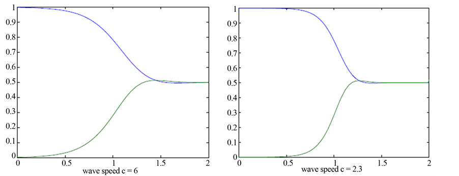
Figure 3. The wave speed c = 6, c = 2.3.
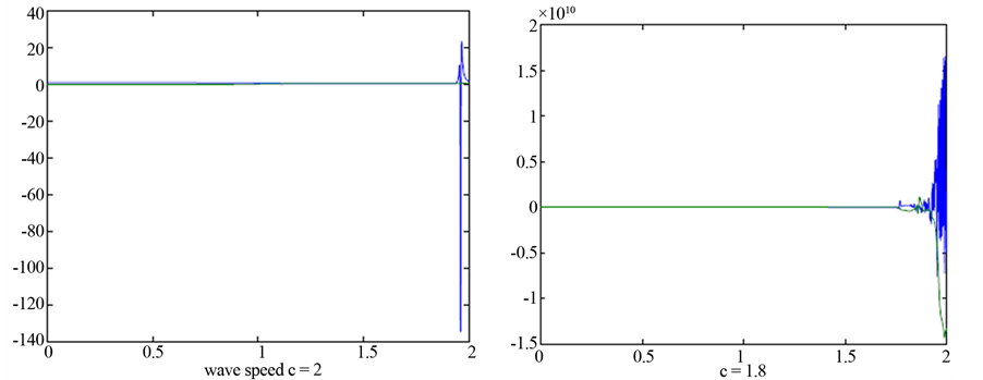
Figure 4. The wave speed c = 2, c = 1.8.
Of course, we mention that the smallest wave speed should exist in between  and
and  by numerical simulation, theoretical proof of the existence of such wave speed seems extraordinarily difficult in this paper and this remains as our future work.
4. Conclusion
In summary, when  sufficiently small, we have obtained the positive equilibrium
  of system (1.2) which is locally asymptotically stable. At the time, we establish the existence of traveling wavefronts of (1.2) connecting
  to
to  .
.
NOTES
*Corresponding author.