Multidimensional Stability of Subsonic Phase Transitions in a Non-Isothermal Van Der Waals Fluid ()
1. Introduction
The motion of a 2-dimensional non-isothermal van der Waals fluid is governed by the following Euler equations
 (1)
(1)
where ,
,  is the density,
  is the velocity with
 , p is the pressure satisfying the following state equation
 (2)
(2)
with  being the specific volume,
  being the temperature, R being the perfect gas constant and a, b being positive constants, e is the specific internal energy given by
 (3)
(3)
and i is the specific enthalpy given by
 (4)
(4)
Otherwise, according to the second law of thermodynamics, the specific entropy s and the specific free energy f of the fluid is defined by
 (5)
(5)
and
 (6)
(6)
respectively. Regarding  as independent variables and denoting
 ,
,


and


where  is the sound speed, we can rewrite (1) as
 (7)
(7)
or
 (8)
(8)
When , the state Equation (2) is not monotonic with respect to
 , which means that there exist
  and
and  such that
 (9)
(9)
The fluid is in liquid phase in the region , while it is in vapor phase in the region
 . The region
  is a highly unstable region (spinodal region) where no state can be found in experiments [2]. Due to such monotonicity, subsonic phase transitions can be found in a van der Waals fluid, which is different from the well-known classical nonlinear waves such as shock waves, rarefaction waves and contact discontinuities.
A subsonic phase transition is a discontinuous solution to the Euler Equation (1) with a single discontinuity, which changes phases across the discontinuity and satisfies certain subsonic condition on both sides of the discontinuity. To explain the concept with more detail, let us consider the following planar subsonic phase transition
 (10)
(10)
where  are constant states of the flow,
  is the constant speed of the discontinuity
  and
and  belong to different phases. The solution (10) satisfies the Rankine-Hugoniot condition
 (11)
(11)
and the subsonic condition
 (12)
(12)
where  denotes the difference of a function across the discontinuity
 ,
,  and
and  are the Mach number and the sound speed on each side of the discontinuity
  respectively.
Due to the subsonic property (12), the well-known Lax entropy inequality [3] is violated for subsonic phase transitions. Hence, several admissibility criteria were introduced to select the physical admissible subsonic phase transitions, among which the viscosity capillarity criterion proposed by Slemrod [4] is an important one. Ever since, for a long time, attention has been paid to isothermal phase transitions and related problems with numerous works devoted to such topics. For problems in one dimensional spaces, see [2,4-6] and references therein. For problems in multi-dimensional spaces, see [7-10] and references therein.
Compared with isothermal phase transitions, there is much less knowledge on non-isothermal phase transitions and there are fewer papers available. Slemrod [11] and Grinfeld [12] proved the existence of traveling waves in Lagrange coordinates by Conley index theory. Hattori [13] considered certain cases of the Riemann problem by the entropy rate criterion. Recently, the author [1] proved the existence and structural stability of traveling waves by using the center manifold method, in light of which, we can expect to reveal more insights of multidimensional phase transitions.
The purpose of this paper is to study the multidimensional stability of non-isothermal phase transitions. With straightforward computation, we show that the corresponding linearized initial boundary problem for the planar phase transition satisfies the uniform Lopatinski condition [14,15]. Without giving much detail, here we briefly state the main result of this paper Theorem 1.1 There exists  and K1 > 0 depending on the bounds of
  and
and  given in (10) and
  given in (18), such that for
  and 0 < K < K1, the
  -admissible phase transition (10) is uniformly stable.
The definitions of the parameters , K,
, K,  and
and  - admissible will be given in Section 2, and the uniform stability will be described in detail in Section 4.
The paper is arranged as follows. Section 2 is a brief recall of the viscosity capillarity criterion for phase transitions and related existence results of traveling waves. In Section 3, we propose the main problem and prove the stability of phase transitions in one dimensional spaces. The multidimensional stability of phase transitions is presented and proved in Section 4.
For the simplicity of notations, we will need the following quantities in the coming arguments.


Considering the planar subsonic phase transition (10), we denote by  the mass transfer flux, and
  and
and . Then, the Rankine-Hugoniot condition (11) and the subsonic condition (12) can be rewritten as
 (13)
(13)
and
 (14)
(14)
respectively.
2. Viscosity Capillarity Profiles
Analogue to the traveling wave method for viscous shocks, the viscosity capillarity criterion is applied to find the planar wave (10) which admits the existence of the following traveling wave
 (15)
(15)
satisfying  and the Navier-Stokes equations
 (16)
(16)
where  is the Laplace operator,
  is the viscosity coefficient,
  is the capillarity coefficient and
  is the heat conductivity coefficient with
 ,
,  ,
, . Substituting (15) into (16) and noticing the Rankine-Hugoniot conditions (11), we can derive the following heteroclinic problem for the unknown functions
 ,
,
 (17)
(17)
where the prime ' denotes the derivative of a function with respect to .
.
In order to deal with the above problem by the center manifold method, we proposed the following assumption in [1],

which was later simplified as
 (18)
(18)
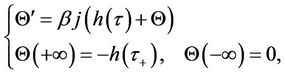
with M being a positive constant and . Employing the Rankine-Hugoniot conditions (13), the hecteroclinic problem (17) becomes
 (19)
(19)
Therefore, the admissibility of subsonic phase transitions can be defined by Definition 2.1 The planar phase transition (10) is admissible if and only if the problem (19) has a solution. The solution  is called the viscosity capillarity profile, or
  -profile for simplicity. The pair
 ,
,  is called
  -admissible.
To state the existence result of  -profile, we will need the following quantities. As usual for fixed
 , the Maxwell equilibrium
  is defined by the equal area rule

Then there exists a unique point , which satisfies that the chord connecting the points
 and
and  is tangent to the graph of
  at the point
  . Denote

When , the
, the  -profile satisfies
 (20)
(20)
which implies . Setting
 , there exists
  satisfying the first equation of (20) by the generalized equal area rule as in [8], which means

Moreover, for every  and
and 
 , a unique pair
  can be found such that
  and
and  can be connected by the
  -profile with the parameters j and
 .
.
Based on the existence of  -profile, the following theorem shows the existence of
  -profile for small
  and small K in [1].
Theorem 2.1 For every  and
and , there exist
 ,
,  and neighborhoods
 ,
,  ,
,  of
of ,
,  ,
,  respectively, such that, for
 , there are unique pair
  and
and , for which
  and
and  are
are  -admissible with the parameters j and
 .
.
Moreover, an additional jump condition can be derived for (10), which plays an essential role in the study of the stability of phase transitions. In the isothermal case [4], due to the subsonic condition (12), the Rankine-Hugoniot condition (11) is not sufficient to guarantee the wellposedness of the boundary value problem for phase transitions, which is also the situation that we encounter in the study of non-isothermal case.
By multiplying the first equation of (19) with  and integrating from
  to
to  with respect to
 , we get the following jump condition on the phase boundary
 (21)
(21)
where


with ,
,  and
and  being the
  -profile with the parameters j and
 .
.
Remark 2.1  is a bounded function which also possesses a uniform limit as
 ,
, . Indeed, from the second equation of (19), we have
where
 .
.
Simple calculation yields

When ,
,  ,
,  has a uniform limit

where  is the
  -profile.
Moreover, from the following jump conditions
 (22)
(22)
the functions  of
of  can be determined by the implicity function theorem for
  near
near  and every
  satisfying the conditions given in Theorem 2.1. The following identities can be easily verified
 (23)
(23)
where − denotes the value of a function for 
 and
and
 ,
,
 ,
,
 .
.
3. Linearized Problems and One Dimensional Stability
In this section, we propose the nonlinear problem for a multidimensional subsonic phase transition and derive the corresponding linearized problem. Then we prove the 1-dimensional stability for the linear problem.
3.1. Linearized Problems
Endow the Euler Equation (1) with the following initial data
 (24)
(24)
where  is the initial discontinuity and
  belong to different phases. If the initial data (24) satisfies certain compatibility conditions, then we can expect to construct the following multidimensional subsonic phase transition
 (25)
(25)
which satisfies the following nonlinear initial boundary value problem
 (26)
(26)
where the third equation is a reformulation of the jump condition (21) with ,
,
 ,
,


and ,
,  satisfying
 .
.
Following [15], we introduce the following transformation to map the free boundary  into a fixed boundary
 (27)
(27)
Then the problem (26) becomes
 (28)
(28)
where we have dropped the tildes for simplicity of notations.
Consider the perturbation,  , of the planar phase transition (10), which satisfies the problem (26) and
 . Denote
 . Then, the following linearized problem for the unknowns
  can be derived from (26),
 (29)
(29)
where

with


and

Remark 3.1 Simple calculation yields

Noticing that the boundary conditions of (29) involve the quantities ,
,  ,
,  and
and , we will need the following lemma to deal with these quantities.
Lemma 3.1 For all , the functions
  and
and  are continuously differentiable. Moreover, their derivatives are continuous with respect to
  at
at  and are bounded depending on the bounds of
  and
and  given in (10) and the constant M given in (18). There exists
  such that for all
 (30)
(30)
Proof. The estimate (30) is immediate from Lemma 2 in [7], once we prove the continuity of . Let us show the continuity of
  and
and . Differentiating (21) with respect to j, we get
 (31)
(31)
By Taylor’s formula, we have


where  and
and  is an infinitesimal as r goes to zero. Substituting the above identities into (31) and employing the calculations (23), we get

which implies
Similar arguments yield the continuity of  and
and  as the following


3.2. One Dimensional Stability
The one dimensional stability concerns the stability of the problem (29) without terms of y-derivatives, namely,
 (32)
(32)
The following theorem shows the stability of planar phase transitions in one dimensional spaces.
Theorem 3.2 There exists  depending on the bounds of
  and
and  given in (10) and the constant
  given in (18), such that for any fixed
  (
( is given in Lemma 3.1.) and
 , the subsonic phase transition (10) is stable with respect to perturbations in the x-direction, which means the problem (32) is well-posed.
Proof. The main idea of the proof is to show that the boundary values of outgoing characteristics and the free boundary can be determined by the boundary conditions, for which we need to investigate the eigenvalues and the eigenvectors of the matrix . The eigenvalues of
  are
are

of multiplicity 1 and

of multiplicity 2. The corresponding right eigenvectors are

and

respectively.
Denote by

the decompositions of  on the bases
respectively. Since the mass transfer flux  is nonzero, we assume
 . Then the subsonic condition (14) becomes
 (33)
(33)
Accordingly, we rewrite the boundary condition of (32) as

to separate the outgoing characteristics together with the free boundary from the incoming characteristics. The necessary and sufficient condition for the well-posedness of the problem (32) is that the determinant
 (34)
(34)
does not vanish. Direct computation yields
 (35)
(35)
where  denotes a bounded term depending on the bounds of
 ,
,  given in (10) and M given in (19). The determinant on the right side of (35) takes the value
for  with
with  given in Lemma 3.1.
Therefore, we can find  depending on the bounds of
 ,
,  given in (10) and the constant
  given in (18) such that for
  and
and ,
,  the problem (32) is well-posed. Similar arguments can be carried out for the case
 .
.
4. Multidimensional Stability
First let us introduce the uniform stability in [15] and state the main result in detail. Denote by

and

the Laplace-Fourier transform of V in  -variables with
 . Then, from (29) we know that
  satisfies
 (36)
(36)
where

and
 .
.
Denote by  all the distinct eigenvalues of
 with multiplicity being mj. Obviously, we have

Introduce

the space of boundary values of all bounded solutions of the special form

to (36) with .
.
Thus, we can state the uniform stability result in detail as follows Theorem 4.1 There exist  and
and  depending on the bounds of
 ,
,  given in (10) and the constant
  given in (18), such that for any fixed
  and
and  the viscosity-capillarity admissible phase transition (10) is uniformly stable, i.e. there is
  such that the estimate
 (37)
(37)
holds for all  and
and .
.
4.1. The Space 
For simplicity, we shall only consider the case

and the other case  can be studied similarly.
Taking the Laplace-Fourier transform on the equation of (29) with  yields
 (38)
(38)
where 
As in [15], if we introduce the transformation
 (39)
(39)
then (38) is equivalent to
 (40)
(40)
where
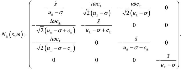
The eigenvalues of  with negative real part for
  are
are

of multiplicity 2 and
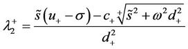
of multiplicity 1, where the  denotes the positive real part square root of a complex value. The corresponding eigenvectors are
 (41)
(41)
 (42)
(42)
and
 (43)
(43)
respectively. The eigenvalue of  with a negative real part for
  is
is

and the corresponding eigenvector is
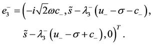 (44)
(44)
Remark 4.1 The above eigenvalues and eigenvectors can be continuously extended to the case . With a little abuse of the notation
 , we still use it to denote those extensions of square roots appearing in the case
 .
.
As in [15], for these vectors, we have Proposition 4.2  are linearly independent for
  and
and  except at
 .
.
In the above cases, the following proposition help us to find the bases of .
.
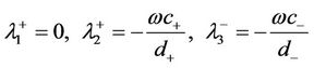
Proposition 4.3 1) If  and
and , then
  and the vectors (41), (44) together with the following eigenvectors


are linearly independent.
2) If  and
and , then
  and the vectors (41), (44) together with the following eigenvectors


are linearly independent.
As in [15], in the critical case , the bases of
  is given by Proposition 4.4 If
  and
and , then
and the corresponding eigenvectors


are linearly independent.
Combining the above propositions, if we naturally expand the eigenvectors as

then the bases of  are given for
  and
and .
.
4.2. Lopatinski Determinant
Now we can show the uniform stability of the phase transition.
Proof of Theorem 4.1. Taking the Laplace-Fourier transformation on the boundary condition in (29) with , multiplying it with the invertible matrix

with  and introducing the transformation (39), we get

where

with


and


To achieve the result, we need to verify the determinant
 (45)
(45)
being nonzero.
Noticing that the eigenvector  remains the same in all the cases mentioned in Section 4.1, the following simplification can be made to
 ,
,
 (46)
(46)
where  is a bounded term depending on the bounds of
 ,
,  given in (10) and
  given in (19),


For sufficiently small , the determinant
  is nonzero as long as the determinant

doesn’t vanish. Considering , one can find that it is similar to the Lopatinski determinant for the corresponding problem in the isothermal case [7,9]. Noticing Proposition 4.2-4.4, we need to consider the following three cases:
1) .
.
We obtain
 (47)
(47)
where
 (48)
(48)
and
 (49)
(49)
Following [9], we claim that  is nonzero for sufficiently small
 .
.
In fact, when , if
, if , then we have
 (50)
(50)
which implies
 (51)
(51)
with  being the Mach numbers. From the subsonic property (12) of the phase transition, we have
 . Due to
 , we deduce that one should take the plus sign in (51), which is not the root of I obviously. Thus, I is always nonzero, which gives that there exist constants
 , and
, and , such that for any
 , we have
 (52)
(52)
When  with
with  and
and , we know that if
  does not equal to the right hand side of (51) with the minus sign, then the inequality (52) holds for any
  with sufficiently small
 . If
. If  satisfies (51) with the minus sign, then the term I vanishes. However, the imaginary part of the term II given in (49) is nonzero, which implies that for any fixed
 , there is a constant
  such that the inequality (52) holds as well.
Therefore, we can find  and
and  depending on
  and
and  given in (10) and the constant
  given in (18) such that
  does not vanish for
  and
and .
.
2) .
.
In this case, we get
 (53)
(53)
which is nonzero for sufficiently small  and
and .
.
3) .
.
In this case, we have
 (54)
(54)
which is also nonzero for sufficiently small  and
and .
.
Therefore, combining the above arguments, we draw the conclusion of the Theorem 4.1.
NOTES
Project 11101076 supported by National Natural Science Foundation of China.
Supported by “The Shanghai Committee of Science and Technology (11ZR1400200)”.