Geometric Inversion of Two-Dimensional Stokes Flows – Application to the Flow between Parallel Planes ()
1. Introduction
Geometric inversion is a type of transformation of the Euclidean plane. This transformation preserves angles and map generalized circles into generalized circles, where a generalized circle means either a circle or a line (a circle with infinite radius). One of the main properties of this method is the transformation of a straight line to a circle. Many difficult problems in geometry become much more tractable when an inversion is applied.
In engineering, the geometric inversion could be very useful to solve complex problems. For example, in fluid mechanics, the equation of two-dimensional Stokes flow remains valid in the new coordinates system obtained by inversion. Thus two-dimensional Stokes flow around certain bodies presenting circular shape appears less difficult to calculate by inversion of flow in channels of parallel walls than by direct calculation using polar coordinates. Although this method is rather general, we will apply it to the case of cellular flows (recirculation flow) presenting viscous eddies. In fact these flows are characterized by the presence of dividing streamlines (separating streamlines) which also give by inversion in the new geometry dividing streamlines.
Much attention has been paid to the steady viscous flow between parallel plates at low Reynolds number (Stokes flow) because of its theoretical importance and also its engineering applications. The particular case of the flow with vanishing velocity to zero when  (i.e. flow with mean rate equal zero) has been widely studied by authors motivated among others by separation phenomena. Thus, after the pioneering work of [1] who presented predictions of cellular motion in Stokes regime between parallel walls, theoretical works like those of [2] and [3] demonstrate the existence of such cellular flow. The corresponding authors showed that, independently of the motion source, any two-dimensional flow with mean rate null in a channel presented necessarily cellular motion composed by successive counter rotating eddies bounded by separating streamlines reattaching the walls. In order to examine the influence of the motion source, accurate computations for various motion sources have been performed [4-16]. Stokes flows and particularly cellular flows could be encountered in numerous applications in physics, biophysics, chemistry and MEMS (Micro and ElectroMechanical Systems) where microflows appear. The particularity of these applications is that they use microchannels [17-19]. Thus, several theoretical and numerical results are available. They could be useful to obtain by inversion transformation the structure and the features of Stokes flows around bodies of circular shape. This transformation is also useful to obtain flow around bodies with complex shape for which the direct calculation could be tiresome.
2. Geometric Inversion-Definitions and Properties
Inversion is the process of transforming points M to a corresponding set of points N known as their inverse points. Two points M and N drawn in Figure 1 are said to be inverses with respect to an inversion circle having inversion centre O and inversion radius R0 if N is the perpendicular foot of the altitude of the triangle OQM, where Q is a point on the circle such that OQ┴QM.
If M and N are inverse points, then the line L through M and perpendicular to OM is called a “polar” with respect to point N, known as the “inversion pole”. In addition, the curve to which a given curve is transformed under inversion is called its inverse curve (or more simply, its “inverse”).
From similar triangles, it immediately follows that the inverse points M and N obey to:
 or
or  (1)
(1)
where the quantity is known as the circle power or inversion power [20].
The general equation for the inverse of the point  relative to the inversion circle with inversion centre
 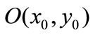 and inversion radius
  is given by
 ,
,  (2)
(2)
Note that a point on the circumference of the inversion circle is its own inverse point. In addition, any angle inverts to an opposite angle.
Treating lines as circles of infinite radius, all circles invert to circles. Furthermore, any two nonintersecting circles can be inverted into concentric circles by taking the inversion centre at one of the two so-called limiting points of the two circles [20], and any two circles can be inverted into themselves or into two equal circles. Or-

Figure 1. Geometric inversion – definition.
thogonal circles invert to orthogonal circles. The inversion circle itself, circles orthogonal to it, and lines through the inversion centre are invariant under inversion. Furthermore, inversion is a conformal map, so angles are preserved. Note that a point on the circumference of the inversion circle is its own inverse point. In addition, any angle inverts to an opposite angle.
The property that inversion transforms circles and lines to circles or lines (and that inversion is conformal) makes it an extremely important tool of plane analytic geometry. Figure 2 shows a simple example of application of geometric inversion.
The circle with dashed lines is the inversion circle of centre O and radius . Let take for example
 , the distance
  and the distance
 . Let’s make inversion of the straight lines L and L’ with centre O and power
 , we obtain the circles C and C’. The points N and Q are respectively the inverse images of the points M and P. The distances ON and OQ, calculated by using Equation (1), are
  and
and . Thus the radii of the circles C and C’ are respectively
  and
and .
.
In Figure 3 we present the classical example of inversion of a square relatively to a circle inscribed in this square. This inversion image becomes more complex if the number of squares is increased (see Mathematica Notebook presenting inversion of a grid).

Figure 2. Inversion of two parallel straight lines.

Figure 3. Inversion of a square. The inversion centre coincides with the square centre.
Figure 4 illustrates the inversion of parabola. This transformation leads to a cardiod defined in Figure 4(c). It’s worth to note that the change of the inversion centre leads to other figures of inversion.