Existence and Multiplicity of Solutions for Quasilinear p(x)-Laplacian Equations in RN ()
1. Introduction
The study of differential and partial differential equations involving variable exponent conditions is a new and interesting topic. The interest in studying such problem was stimulated by their applications in elastic mechanics and fluid dynamics. These physical problems were facilitated by the development of Lebesgue and Sobolev spaces with variable exponent.
The existence and multiplicity of solutions of  -Laplacian problems have been studied by several authors (see for example [1] [2] , and the references therein).
In [3] , A. R. EL Amrouss and F. Kissi proved the existence of multiple solutions of the following problem
 (1)
(1)
Also Xiaoyan Lin and X. H. Tang in [4] studied the following quasilinear elliptic equation
 (2)
(2)
and they proved the multiplicity of solutions for problem (2) by using the cohomological linking method for cones and a new direct sum decomposition of .
.
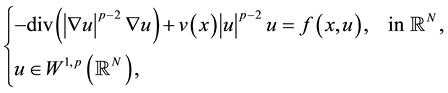
In this paper, we consider the following problem
 (3)
(3)
where  is the
  -Laplacian operator;
  is a Lipschitz continuous function with
 is a given continuous function which satisfies
(B0)
here m is the Lebesgue measure on RN.
 is a Carathéodory function satisfying the subcritical growth condition
(F0)
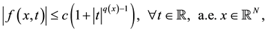
for some , where
 ,
,  ,
, ![]() , and
, and
![]()
Define the subspace
![]()
and the functional![]() ,
,
![]()
where![]() .
.
Clearly, in order to determine the weak solutions of problem (3), we need to find the critical points of functional Φ. It is well known that under (B0) and (F0), Φ is well defined and is a C1 functional. Moreover,
![]()
for all![]() .
.
If ![]() for a.e.
for a.e.![]() , the constant function
, the constant function ![]() is a trivial solution of problem (3). In the following, the key point is to prove the existence of nontrivial solutions for problem (3).
is a trivial solution of problem (3). In the following, the key point is to prove the existence of nontrivial solutions for problem (3).
Set
![]() (4)
(4)
This paper is to show the existence of nontrivial solutions of problem (3) under the following conditions.
(F1)
![]()
where ![]() as given in (4).
as given in (4).
(F2) There exist ![]() and
and![]() , such that
, such that
![]()
(F3) There exist ![]() and
and ![]() such that
such that
![]()
for a.e.![]() .
.
(F4) ![]() as
as ![]() and uniformly for
and uniformly for![]() , with
, with![]() . Here
. Here ![]() is given in the condition (F0).
is given in the condition (F0).
We have the following results.
Theorem 1.1. If ![]() satisfies (B0),
satisfies (B0), ![]() satisfies (F0), (F1) and (F2), then problem (3) possesses at least one nontrivial solution.
satisfies (F0), (F1) and (F2), then problem (3) possesses at least one nontrivial solution.
Theorem 1.2. Assume ![]() satisfies (B0),
satisfies (B0), ![]() satisfies (F0), (F3) and (F4), with
satisfies (F0), (F3) and (F4), with ![]() for a.e.
for a.e.![]() , then problem (3) has at least two nontrivial solutions, in which one is non-negative and another is non-positive.
, then problem (3) has at least two nontrivial solutions, in which one is non-negative and another is non-positive.
This paper is divided into three sections. In the second section, we state some basic preliminary results and give some lemmas which will be used to prove the main results. The proofs of Theorem 1.1 and Theorem 1.2 are presented in the third section.
2. Preliminaries
In this section, we recall some results on variable exponent Sobolev space ![]() and basic properties of the variable exponent Lebesgue space
and basic properties of the variable exponent Lebesgue space![]() , we refer to [5] -[8] .
, we refer to [5] -[8] .
Let![]() ,
,![]() . Define the variable exponent Lebesgue space:
. Define the variable exponent Lebesgue space:
![]()
For![]() , we define the following norm
, we define the following norm
![]()
Define the variable exponent Sobolev space:
![]()
which is endowed with the norm
![]()
It can be proved that the spaces ![]() and
and ![]() are separable and reflexive Banach spaces. See [9] for the details.
are separable and reflexive Banach spaces. See [9] for the details.
Proposition 2.1. [10] [11] Let
![]()
Then we have
1) For![]() ,
,![]() ;
;
2)![]() ,
, ![]()
3) ![]()
4)![]() ,
, ![]()
For ![]() with
with![]() , let
, let ![]() satisfy
satisfy
![]()
We have the following generalized Hölder type inequality.
Proposition 2.2. [9] [12] For any ![]() and
and![]() , we have
, we have
![]()
We consider the case that ![]() satisfies (B0). Define the norm
satisfies (B0). Define the norm
![]()
Then ![]() is continuously embedding into
is continuously embedding into ![]() as a closed subspace. Therefore,
as a closed subspace. Therefore, ![]() is also a separable and reflexive Banach space.
is also a separable and reflexive Banach space.
Similar to the Proposition 2.1, we have
Proposition 2.3. [13] The functional ![]() defined by
defined by
![]()
has the following properties:
1)![]() ;
;
2) ![]()
3) ![]()
Lemma 2.4. [13] If ![]() satisfies (B0), then
satisfies (B0), then
1) we have a compact embedding![]() ;
;
2) for any measurable function ![]() with
with![]() , we have a compact embedding
, we have a compact embedding
![]() . Here
. Here ![]() means that
means that![]() .
.
Now, we consider the eigenvalues of the p(x)-Laplacian problem
![]() (5)
(5)
For any![]() , define
, define ![]() by
by
![]()
For all![]() , set
, set
![]()
then ![]() is a
is a ![]() submanifold of E since t is a regular value of H. Put
submanifold of E since t is a regular value of H. Put
![]()
where ![]() is the genus of I.
is the genus of I.
Define
![]()
We denote by ![]() the eigenpair sequences of problem (5) such that
the eigenpair sequences of problem (5) such that
![]()
![]()
Define
![]()
![]()
![]() , where
, where![]()
Lemma 2.5. For all![]() , let
, let ![]() be an eigenfunction associated with
be an eigenfunction associated with ![]() of the problem (5). Then,
of the problem (5). Then,
![]()
Proof. Let![]() . From the definition of
. From the definition of![]() , it is easy to see that
, it is easy to see that![]() .
.
On the other hand, since the functional ![]() is coercive and weakly lower semi-continuous and
is coercive and weakly lower semi-continuous and ![]() is weakly closed subset of E, there exists
is weakly closed subset of E, there exists ![]() such that
such that![]() . Letting
. Letting![]() , then
, then ![]() and
and![]() . Thus the lemma follows. ,
. Thus the lemma follows. ,
Lemma 2.6.
![]()
Proof. From Lemma 2.5, we have
![]()
Since
![]()
so we have ![]() Then,
Then,
![]()
Thus we get ![]() and
and![]() .
.
Similarly, if ![]() is the eigenfunction associated with
is the eigenfunction associated with![]() , we get
, we get ![]() and
and![]() . Finally, we obtain
. Finally, we obtain ![]()
On the other hand, it is easy to see that ![]() Thus the lemma follows. ,
Thus the lemma follows. ,
Now, we consider the truncated problem
![]()
where
![]()
We denote by ![]() and
and ![]() the positive and negative parts of u.
the positive and negative parts of u.
Lemma 2.7.
1) If ![]() then
then ![]() and
and
![]()
2) The mappings ![]() are continuous on E.
are continuous on E.
Lemma 2.8. All solutions of ![]() (resp.
(resp.![]() ) are non-positive (resp. non-negative) solutions of problem (3).
) are non-positive (resp. non-negative) solutions of problem (3).
Proof. Define ![]()
![]()
where ![]() From Lemma 2.7 and (F0),
From Lemma 2.7 and (F0), ![]() is well defined on E, weakly lower semi-con- tinuous and C1-functionals.
is well defined on E, weakly lower semi-con- tinuous and C1-functionals.
Let u be a solution of![]() . Taking
. Taking ![]() in
in
![]()
we have
![]()
By virtue of Proposition 2.3, we have![]() , so
, so ![]() and
and![]() , a.e.
, a.e.![]() , then u is also a critical point of the functional Φ with critical value
, then u is also a critical point of the functional Φ with critical value![]() .
.
Similarly, the nontrivial critical points of the functional ![]() are non-negative solutions of problem
are non-negative solutions of problem![]() . ,
. ,
3. Proof of Main Results
3.1. Proof of Theorem 1.1
To derive the Theorem 1.1, we need the following results.
Proposition 3.1. Φ is coercive on E.
Proof. Put
![]()
From (F1) we have, for any![]() , there is
, there is ![]() such that
such that
![]()
By contradiction, let ![]() and
and ![]() such that
such that
![]() (6)
(6)
Putting![]() , one has
, one has![]() . For a subsequence, we may assume that for some
. For a subsequence, we may assume that for some![]() , we have
, we have
![]() weakly in E and
weakly in E and ![]() strongly in
strongly in![]() .
.
Consequently,![]() . Let
. Let![]() , via the result above we have
, via the result above we have ![]() and
and
![]()
Set
![]()
then,
![]()
From (6), (F1) and Lemma 2.6, we deduce that
![]()
This is a contradiction. Therefore, Φ is coercive on E. ,
Proposition 3.2. Assume ![]() satisfies (F0) and (F2), then zero is local maximum for the functional
satisfies (F0) and (F2), then zero is local maximum for the functional![]() ,
, ![]() ,
,![]() .
.
Proof. From (F2), there is a constant ![]() such that
such that
![]() (7)
(7)
From (F0) and![]() , there exists
, there exists ![]() such that
such that
![]() (8)
(8)
By (7) and (8), we get
![]() (9)
(9)
For ![]() we have
we have
![]()
Since![]() , there is a
, there is a ![]() such that
such that
![]() (10)
(10)
Thus the proposition follows. ,
Proof of Theorem 1.1. From Proposition 3.1, we know Φ is coercive on E. Since Φ has a global minimizer ![]() on E, Φ is weakly lower semi-continuous and
on E, Φ is weakly lower semi-continuous and![]() , then, in order to prove
, then, in order to prove![]() , we need to prove
, we need to prove![]() . So we have the Theorem 1.1 following from Proposition 3.2. ,
. So we have the Theorem 1.1 following from Proposition 3.2. ,
3.2. Proof of Theorem 1.2
To find the properties of the p(x)-Laplacian operators, we need the following inequalities (see [10] ).
Lemma 3.3. For ![]() and
and ![]() in RN, then there are the following inequalities
in RN, then there are the following inequalities
![]()
Proposition 3.4. Assume (F0), and let ![]() be a sequence such that
be a sequence such that ![]() in E and
in E and ![]() for all
for all ![]() as
as![]() , then, for some subsequences,
, then, for some subsequences, ![]() , a.e. in RN, as
, a.e. in RN, as ![]() and
and ![]() for all
for all![]() .
.
Proof. Let ![]() and
and ![]() such that
such that
![]()
Let us denote by ![]() the following sequence
the following sequence
![]()
From Lemma 3.3, we have ![]() and
and
![]()
Recalling that ![]() in E, we get
in E, we get
![]()
and so,
![]() (11)
(11)
On the other hand, by (11) and ![]() we obtain
we obtain
![]()
Thus,
![]()
Combining Hölder’s inequality and Sobolev embedding, we deduce that
![]() (12)
(12)
Let us consider the sets
![]()
From Lemma 3.3, we get
![]() (13)
(13)
![]() (14)
(14)
Applying again Hölder’s inequality,
![]() (15)
(15)
where
![]()
and
![]()
Then,
![]() (16)
(16)
From (12) and (13), we have
![]() (17)
(17)
By (15)-(17), we obtain
![]() (18)
(18)
(12) and (14) imply that
![]() (19)
(19)
From (18) and (19), ![]() a.e. in
a.e. in![]() . Because R is arbitrary, it follows that for some subsequence
. Because R is arbitrary, it follows that for some subsequence
![]() .
.
Combined with Lebesgue’s dominated convergence theorem, we get
![]() (20)
(20)
By (20) and![]() , we derive that
, we derive that ![]() for all
for all![]() . ,
. ,
Proposition 3.5. Assume (F0), and let ![]() and
and ![]() be a (PS)d sequence in E for
be a (PS)d sequence in E for ![]() then
then ![]() is bounded in E.
is bounded in E.
Proof. From (F0), we have ![]() It is clear that
It is clear that
![]()
Assume that ![]() for some
for some![]() , then, by Proposition 2.3, Hölder’s inequality and Sobolev embedding, we have
, then, by Proposition 2.3, Hölder’s inequality and Sobolev embedding, we have
![]() (21)
(21)
Since ![]() and
and![]() , (21) implies that
, (21) implies that ![]() is bounded in E. ,
is bounded in E. ,
Proposition 3.6. Assume ![]() satisfies (B0),
satisfies (B0), ![]() satisfies (F0) and (F4), and let
satisfies (F0) and (F4), and let ![]() be a (PS)d sequence in E, then
be a (PS)d sequence in E, then ![]() satisfies the (PS) condition.
satisfies the (PS) condition.
Proof. From Proposition 3.4, we have
![]() (22)
(22)
By Lemma 2.4, we get
![]() (23)
(23)
On the other hand, Lebesgue’s dominated convergence theorem and the weak convergence of ![]() to u in E show
to u in E show
![]() (24)
(24)
Moreover, since ![]() are bounded in
are bounded in![]() , then we have
, then we have
![]()
Therefore, by virtue of the definition of weak convergence, we obtain
![]() (25)
(25)
By (23)-(25), we have
![]() (26)
(26)
By (22) and (26), we get
![]()
Then combining Lemma 3.3, we obtain
![]()
which imply that ![]() in E. ,
in E. ,
Proposition 3.7. There exist ![]() and
and ![]() such that
such that![]() , for all
, for all ![]() with
with![]() .
.
Proof. The conditions (F0) and (F4) imply that
![]()
For ![]() small enough, combined with Proposition 2.3, we have
small enough, combined with Proposition 2.3, we have
![]() (27)
(27)
By the condition (F0), it follows
![]()
from Lemma 2.4, which implies the existence of ![]() such that
such that
![]() (28)
(28)
Using (28) and Proposition 2.1, we deduce
![]()
Combining (27), it results in that
![]()
here ![]() are positives constants. Taking
are positives constants. Taking ![]() such that
such that ![]() we obtain
we obtain
![]()
Since![]() , the function
, the function ![]() is strictly positive in a neighborhood of zero. It follows that there exist
is strictly positive in a neighborhood of zero. It follows that there exist ![]() and
and ![]() such that
such that
![]()
,
Proposition 3.8. If ![]() and
and![]() , we have
, we have ![]() for a certain
for a certain![]() .
.
Proof. From the condition (F3), we get
![]()
For ![]() and
and![]() , we have
, we have
![]()
Since![]() , we obtain
, we obtain
![]()
,
Proof of Theorem 1.2. According to the Mountain Pass Lemma, the functional ![]() has a critical point
has a critical point ![]() with
with![]() . But,
. But, ![]() , that is,
, that is, ![]() , a.e.
, a.e.![]() . Therefore, the problem
. Therefore, the problem ![]() has a nontrivial solution which, by Lemma 2.8, is a non-positive solution of the problem (3).
has a nontrivial solution which, by Lemma 2.8, is a non-positive solution of the problem (3).
Similarly, for functional![]() , we still can show that there exists furthermore a non-negative solution. The proof of Theorem 1.2 is now complete. ,
, we still can show that there exists furthermore a non-negative solution. The proof of Theorem 1.2 is now complete. ,
Acknowledgements
This work has been supported by the Natural Science Foundation of China (No. 11171220) and Shanghai Leading Academic Discipline Project (XTKX2012) and Hujiang Foundation of China (B14005).