On the Lagrange Stability of Motion and Final Evolutions in the Three-Body Problem ()
1. Introduction
It is known [2-4] that the three-body problem (for mass points) is considered for the system of three bodies with masses  respectively, that are in the movement in the three-dimensional Euclidean space under the mutual gravitational attraction. We have to determine their coordinates and velocities at any time
  on the base of initial data. In this form, despite of significant progress based on the achievements of KolmogorovArnold-Moser theory [5], the problem remains unsolved until now, and therefore a qualitative study of motion in this system is still important. In particular, it is still important to obtain an answer for the following question: What are conditions under which three bodies remans inside a bounded domain of the Euclidean space. Later, we will suggest sufficient conditions for the boundedness of the motion.
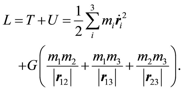
Before we start to investigate the motion of the mass points, we write down the formula for the related Lagrangian:
 (1.1)
(1.1)
Here,  are radius vectors of points in the inertial reference system with the origin at the center of masses
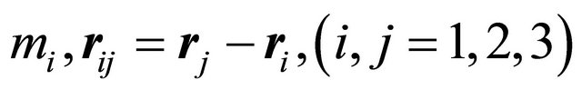 ,
, is the gravitation constant. The motion equations for the Lagrangian (1.1) take the following form
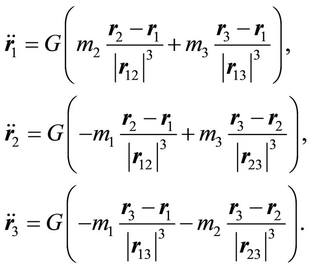 (1.2)
(1.2)
Passing over to dimensionless time variable
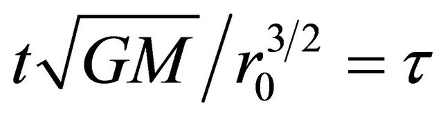
in (1.2), where 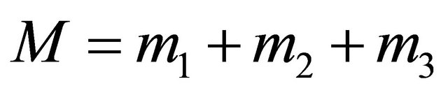 and
and  is a parameter with the dimension of the length unit, we obtain the following equations [6]
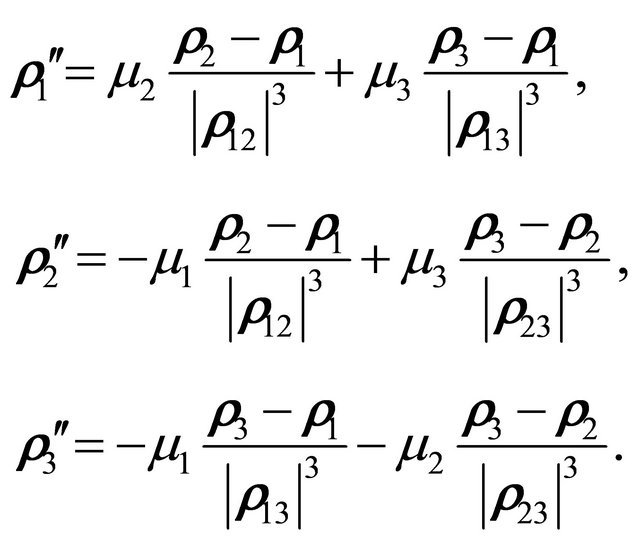 (1.3)
(1.3)
Here, the prime sign denotes the differentiation with respect to ,
,  are relative radius vectors.
In what follows, along with Equations (1.3), we will use the following equations for distances that were obtained in [6]:
 (1.4)
(1.4)
where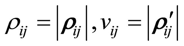 .
.
The system of ten Equations (1.4) is an integral manifold (i.e., a subset) of system (1.3) and it is useful in the study of orbital stability of motions.
In what follows, we will also use the integral of energy
 (1.5)
(1.5)
and the vector integral of angular momentum
 (1.6)
(1.6)
Next, we will always assume that .
.
Since, additionally, there are integrals of motion for the center of mass for this system, without loss of generality in what follows we can assume in accordance with the choice of coordinate system that
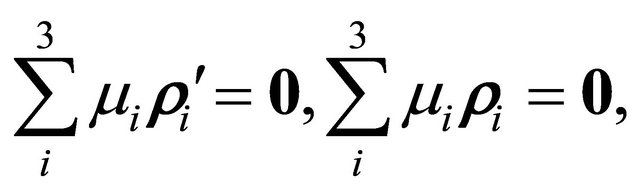 (1.7)
(1.7)
and, as a consequence [3,7,8],
 (1.8)
(1.8)
Finally, we will also use obtained in [1], as a consequence of (1.7), the following equations:
 (1.9)
(1.9)
By reversing Equations (1.9), we have
 (1.10)
Here . Similar equations connect
  and
and  [1].
[1].
Based on the key equations and equalities obtained above, further in Section 2 we suggest the basic definitions and auxiliary statements. These definitions and statements form the foundation to achieve our main goal that is to prove Theorem 1 on the Lagrange stability in Section 3.
Theorem 1, which in our view has an intrinsic interest, is important because of its corollary that reveals important details of hyperbolic-elliptic and parabolic-elliptic final evolutions, which will be touched upon in Section 4.
2. Main Definitions and Assumptions
Definition 1. We say that the motion
 of system (1.3) is Lagrange stable if the following condition is satisfied:
 (2.1)
(2.1)
where  are positive constants.
Definition 2. We say that the motion
 of system (1.3) is distal if the following inequality is satisfied:
 (2.2)
(2.2)
As it was mentioned above, Equations (1.3) contain relative radius vectors  where
where  is a parameter that has the dimension of the length unit. Therefore, without loss of generality in what follows, it is convenient for us to put
  at a value, for which we have
  in inequalities (2.1) and (2.2).
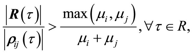
Definition 3. In accordance with [9], we say that a fixed pair of points  of system (1.3) is Hill stable if the following inequality is satisfied:
 (2.3)
(2.3)
Definition 4. In accordance with [9], we say that a fixed pair of mass points , of system (1.3) is Hill absolutely stable if the following inequality is satisfied:
 (2.4)
(2.4)
where  denotes distance from third mass point to the center of mass of fixed pair of points
 .
.
As it is proved in [9], if a fixed pair of mass points , of system (1.3) is Hill absolutely stable, then it is Hill stable and collisions are possible only for mass points, which form this fixed pair.
Key points for forming of initial conditions, under which we have the Hill stability of a pair of mass points, are integrals of energy and angular momentum [9-11].
Lemma 1. If one of the pairs of mass points in the three-body problem is Hill stable, then there exists a closed ball  in the appropriate configuration space
  such that none of the vectors
  in
in  can be a zero vector.
Proof. The lemma is obvious when it comes to the triple collision. Therefore, in what follows, we restrict ourselves to the case where only one of the vectors  is a zero vector.
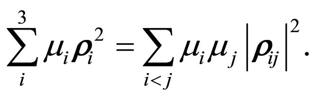
As it is known (see e.g. [12]), the following relations are valid:
 (2.5)
(2.5)
Suppose that . Then due to the first relation of system (2.5) we have
 (2.6)
(2.6)
Supplementing equality (2.6) with the identity
 (2.7)
(2.7)
we obtain
 (2.8)
(2.8)
and these relations show that if at least one of the distances  is bounded, then all three distances are bounded.
If we have either the equality  or the equality
  instead of
 , we argue similarly.
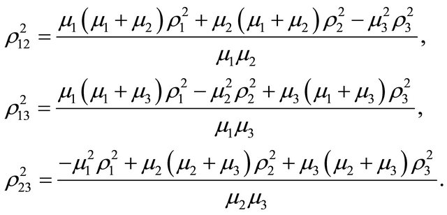
In what follows, without loss of generality, we assume that the Hill stable pair is the pair . Then, by using equalities (1.9), in dependence of which one of the vectors
  is a zero vector, we obtain three different expressions for the radius of the ball that is referred to the center of mass of three particles:
 (2.9)
(2.9)
Equalities (2.9) allow us to conclude that if one of the vectors  is zero vector, then motions can be embedded into a closed ball
  with the radius defined by relations
 (2.10)
The Lemma 1 is proved.
Corollary 1. The scheme of the proof of Lemma 1 implies that the radius  of the sphere
  can always be chosen not only in such a way that each of the variables
  is not vanish in
 , but also to exceed some positive constant.
Corollary 2. If the motion in the three-body problem is outgoing, then surely there is a time  such that the segment of the orbit (the projection of the phase trajectory in the configuration space) falls into
  for
for .
.
Lemma 2. Let  be a Lagrange unstable motion of system (1.3), for which the pair of bodies
  is Hill absolutely stable.
Then, for this motion, there is a sequence

such that the equalities
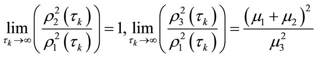 (2.11)
are valid.
Proof. Since the motion under consideration is Lagrange unstable, there is a sequence

such that
 (2.12)
Let us divide the first equality of system (1.10) by . As a result, for the Lagrange unstable motion we have
 (2.13)
Tending  to infinity in equality (2.13), we obtain the equality
 (2.14)
Further, on the base of last two equalities of system (1.10), we derive
 (2.15)
Observing
and taking into account (1.8), (2.12), we obtain
 (2.16)
In the limit, on the base of (2.15), (2.16), we have
 (2.17)
By Equations (2.14), (2.17) we derive

Lemma 2 is proved.
Lemma 3. Let  be a distal and Lagrange unstable motion of system (1.3), for which the pair of bodies
  is Hill stable.
Then, there is a sequence  such that in the limit case one of the equalities
 (2.18)
 (2.19)
 (2.20)
is valid.
Proof. Since the motion under consideration is Lagrange unstable, there is a sequence  such that
 (2.21)
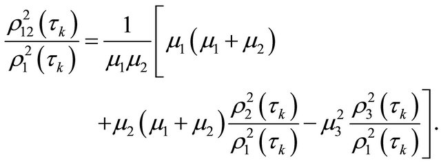
We rewrite equalities (1.9) in the following form:
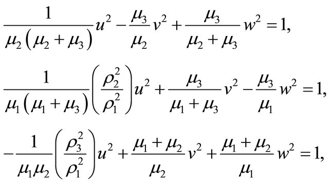 (2.22)
where
 (2.23)
As a result, we obtain a system of three equations that are linear with respect to  and contain variable coefficients
  and
and , and each one of these equations can be treated as an equation of a onesheet hyperboloid. Moreover, if the first equation describes a stationary hyperboloid, then the second and the third ones describe movable hyperboloids, if we take into account the fact that coefficients
  and
and  are variable. All these hyperboloids have distinct imaginary semiaxes.
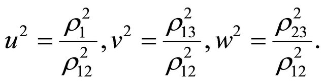
Let us exclude the variable  from Equations (2.22). As a result, we obtain equations
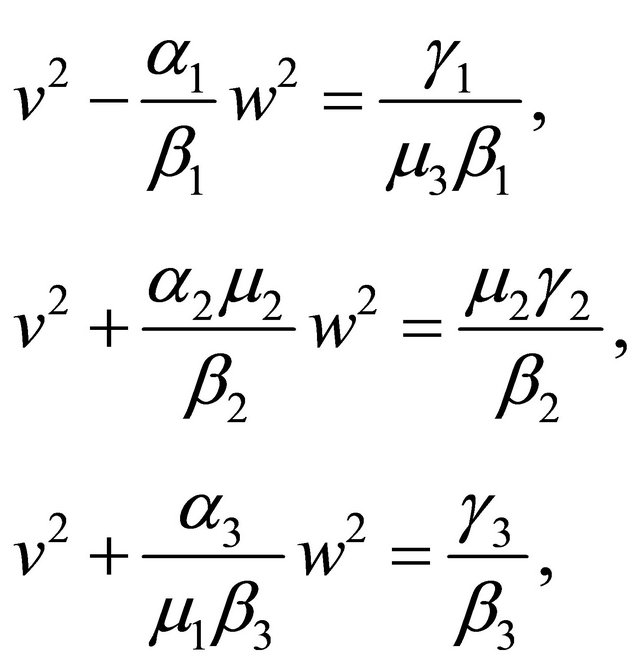 (2.24)
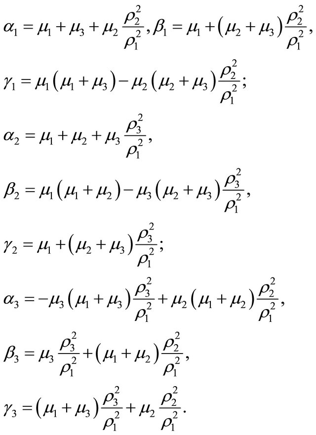
where
Under the conditions of Lemma 3, the considerable movement is Lagrange unstable. Hence, in accordance with Lemma 2, variable coefficients  and
and  satisfy equalities (2.11) with
 .
.
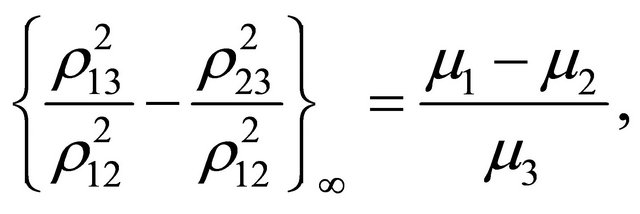
Let us consider the limit version of Equations (2.24) when . Taking equalities (2.11) into account, in the limit case, on the base of (2.24) we obtain equalities (2.18)-(2.20). Since the system (2.18)- (2.20), which is treated as a system of linear equations with respect to variables
  and
and , is inconsistent, we conclude that only one of equalities (2.18)-(2.20) for considerable motion is valid.
Lemma 3 is proved.
3. A Theorem on Lagrange Stability
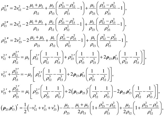
Let us try to use the information obtained in the previous section in order to carry out a qualitative analysis of the movement equations. In this connection, it should stressed that distance Equations (1.4) from the first section contain the term
Along with this fact, similar terms are contained in the left-hand sides of Equations (2.18)-(2.20), though, it is true in the limit case where we assume that the movement under consideration is Lagrange unstable. Hence, there is a point in considering a hypothetical possibility of the Lagrange unstable movement in the case of obtained movement equations hoping that we obtain some useful information about qualitative behavior of movements in the system. To this end we represent movement Equation (1.3) in the form
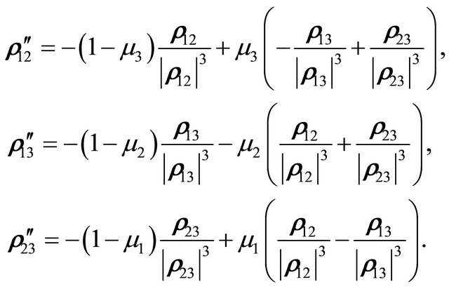 (3.1)
(3.1)
Equations (3.1) are more appropriate for our further purposes, though Equations (1.3) will be still considered as basic ones.
Theorem 1. Let  be a distal movement of system (1.3) that belongs to the set
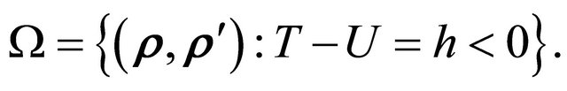
Then, if masses  are different and one of the pairs of the mass points is Hill stable, then the movement under study is Lagrange stable.
Proof. Without loss of generality we can assume that the pair  is Hill stable.
Suppose that under the conditions of the theorem the movement  is Lagrange unstable. Then there exist a sequence
  such that
 (3.2)
(3.2)
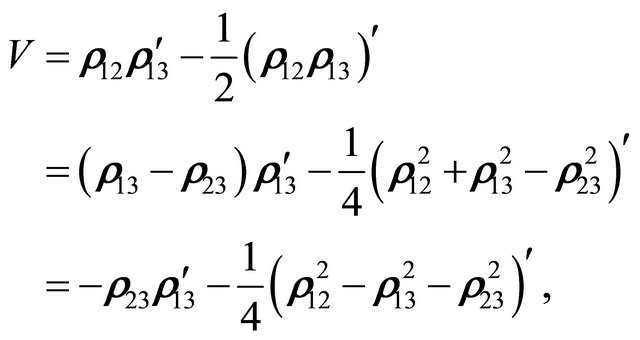
Let us consider the function
 (3.3)
(3.3)
which is formed on the base of the structure of the system of Equations (1.4). Its derivative with respect to the vector field, which is determined by Equations (3.1), has the form
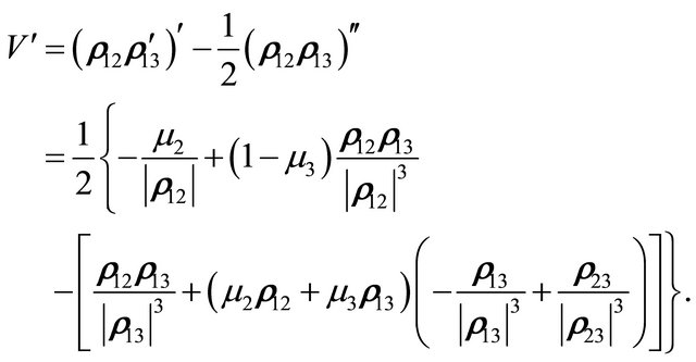 (3.4)
(3.4)
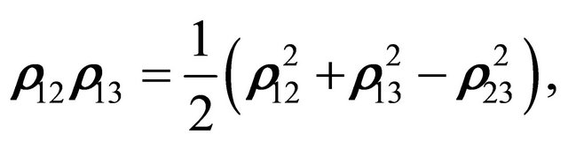
Noticing that
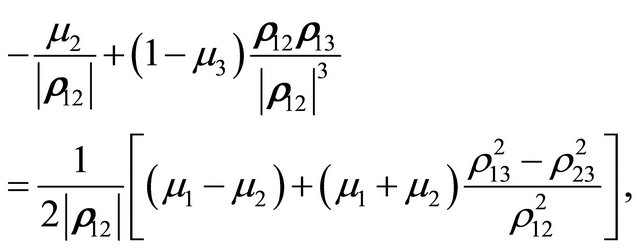
we can rewrite equality (3.4) in the form
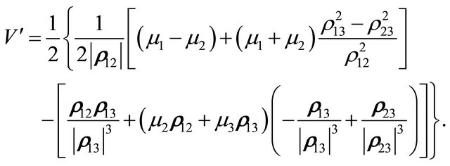 (3.5)
(3.5)
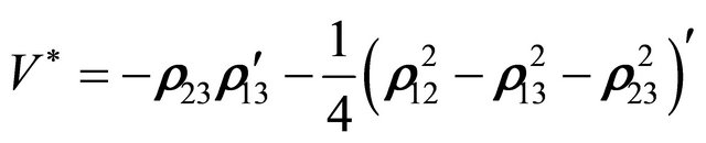
Assuming that the movement under study is Lagrange unstable and taking into account equalities (3.2), on the base of (3.5) we obtain in the limit case that
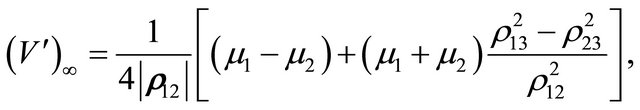 (3.6)
(3.6)
By equality (3.6), considering equalities (2.18)-(2.20), we derive
 (3.7)
(3.7)
 (3.8)
(3.8)
 (3.9)
(3.9)
The upper indices 1, 2, 3 in the left-hand sides of equalities (3.7)-(3.9) mean that instead of
in the right-hand side of equality (3.6) we substitute expressions that are determined by right-hand sides of equalities (2.18), (2.19), (2.20) respectively.
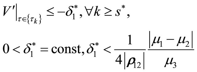
First let us consider equality (3.7), for which we assume that  and hence, we assume that the righthand side of equality (3.7) is positive. As a consequence of this fact, on the base of continuity of the right-hand side of equality (3.5) we can conclude that, for the sequence
 , there is a sufficiently large number
  such that the inequality
 (3.10)
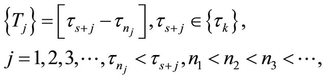
takes place for . In accordance with conditions of the theorem, the movement under study is distal, and hence velocities of mass points are bounded. From this fact we can conclude that there is a sequence of time intervals with growing lengths
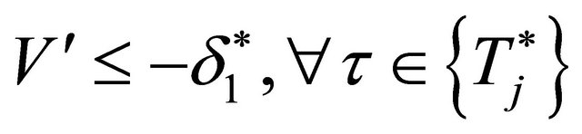
for which we have the inequality
 (3.11)
By integrating (3.11), we obtain the inequality
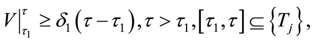
which can be further rewritten in the form
 (3.12)
The product  is bounded on
  due to conditions of the theorem. Therefore, by replacing it with a certain relevant constant
 , we can strengthen equality (3.12):
 (3.13)
By integrating inequality (3.13), we obtain
 (3.14)
Let us set  in inequality (3.14) and rewrite it in the form
 (3.15)
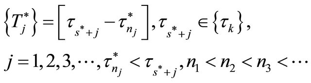
The terms

in (3.15) correspond to finite time points  such that the sum
  reach a critical value at which we have
Hence, the quantities
in inequality (3.15) can be always chosen in such a way that they are finite. Relating to this fact, it is appropriate for us to rewrite inequality (3.15) in the form
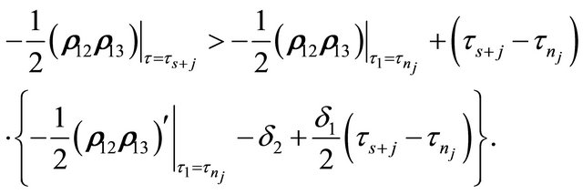 (3.16)
In accordance with (3.2) and the definition of time points , the length of the interval
  tends to infinity as
 . Hence, the right-hand side of inequality (3.16) tends to infinity as well.
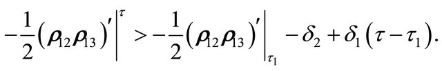
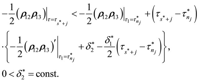
Now let us analyze the left-hand side of inequality (3.16) in a more detailed way. To this end we note that
and represent it in the form
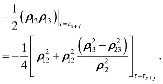 (3.17)
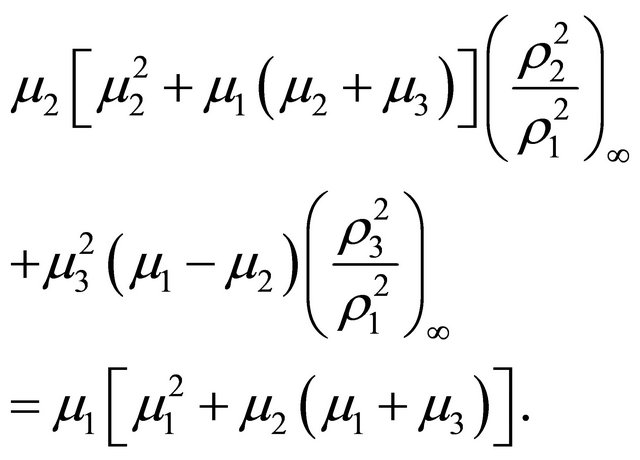
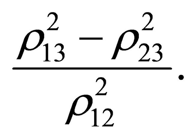
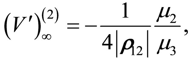
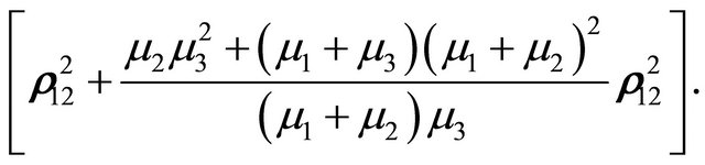
As  tends to infinity, by equality (2.18) the terms inside the square brackets tend to the expression
 (3.18)
Thus, in accordance with our assumption , the left-hand side of inequality (3.16) tends to a negative value as
 . We arrive to a contradiction.
So, if equality (3.7) holds true and , then the assumption on the Lagrange instability of the movement
  is not true.
In an absolutely similar way we can obtain a contradiction in the case where equality (3.9) is satisfied. Note only the fact that an analogue of expression (3.18) in this case is the expression
Now consider Equation (3.7) in the case where , and hence, its right-hand side is negative. In this case, similarly to the case that was studied above, due to continuity of the right-hand side of equality (3.5) we can assert for the sequence
  that there exist a sufficiently large number
  such that the inequality
 (3.19)
takes place for . From this, by distality of the motion, we can conclude similarly to the case studied above that there exist a sequence of time intervals
with growing lengths for which the inequality
 (3.20)
is satisfied.
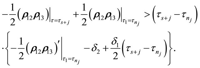
By using almost literally the same scheme of arguments that was used for equality (3.7) in the case where , we arrive to an analogue of inequality (3.16):
 (3.21)
Due to (3.18), we can conclude that, as , the left-hand side of inequality (3.21) tends to a bounded value and the right-hand side tends to minus infinity. Hence, we arrive to a contradiction.
Thus, the assumption on the Lagrange instability of the movement under study is also not true in the case where equality (3.7) is valid as .
.
Finally, it remains to consider the case where equality (3.8) is satisfied. In this case, we can apply the arguments that were used for Equation (3.7) under the condition . It should be note only the fact that an analogue of expression (3.18) in this case will be represented by the expression
Thus, if we assume that the movement under study is Lagrange unstable, then we arrive to a contradiction in all three cases where equalities (3.7)-(3.9) take place. This contradiction give us a possibility to conclude that the theorem is true.
Remark 1. As it is implied by the structure of Equations (1.4) and the scheme of proof of Theorem 1, the Lagrange stability remains to be true also in the case where only different masses are ones that form a Hill stable pair. For the third particle, it is admissible that its mass is equal to the mass of a particle from the Hill stable pair.
Remark 2. If we take into account the fact that
then we can consider the derivative of the function
with respect to the vector field that is determined by Equations (1.4). However the function  in the form (3.3) is more appropriate. It is the function
  in the form (3.3) which is predetermining the use of Equations (3.1), though in the construction of the function
  we are based on the structure of the system of Equations (1.4).
4. On Hyperbolic-Elliptic and Parabolic-Elliptic Final Evolutions
As it is known [13], hyperbolic-elliptic and parabolicelliptic final evolutions are accompanied by a motion of a bounded pair of particles and the third outgoing remote particle. In this case, we can apply Lemma 2 in order to conclude that relations (2.11) take place.
By using the Jacobi decomposition, we can represent the motion of the bounded pair in the following convenient form:
 (4.1)
(4.1)
Here, as it is usual, we have  and
and  denotes the distance from the third mass point to the center of masses of the pair
 . As we can see, vector equation (4.1) represents the two-body problem with a decreasing perturbation since the third particle is outgoing.
Since , we see that
  tends to the elliptic Kepler motion with the relevant limit integrals of the motion [10]:
 (4.2)
(4.2)
 (4.3)
(4.3)
Let  denote the asymptotic Kepler motion with integrals
  and
and . In this case, in accordance with [10], we have
 (4.4)
(4.4)
if the evolution is hyperbolic-elliptic, and
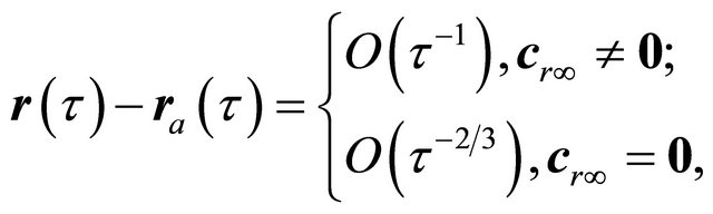 (4.5)
(4.5)
if the evolution is parabolic-elliptic.
It turns out that Theorem 1 provides a possibility to correct equalities (4.4) and (4.5) respectively. In particular, we can obtain the following statement.
Corollary of Theorem 1. Let masses  in the three-body problem be different and
 . Then in cases of hyperbolic-elliptic and parabolicelliptic final evolutions, the following equalities are respectively valid:
 (4.6)
(4.6)
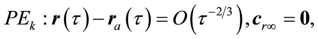 (4.7)
(4.7)
i.e., going over to the limit, the modulus of the angular momentum  of the bounded pair
  can not exceed a positive constant.
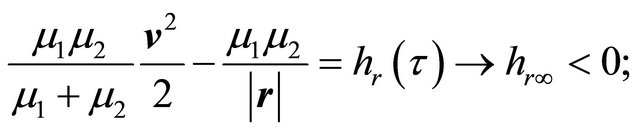
Proof. Let us suppose the contrary,  , and consider the limit energy integral for the pair
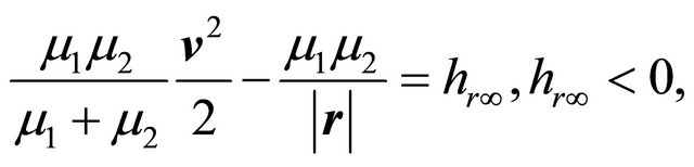 (4.8)
(4.8)
which, in its turn, can be rewritten in the form
 (4.9)
(4.9)
Since , due to (4.9) we have

and this implies
 (4.10)
In accordance with inequality (4.10), we conclude that if , then hyperbolic-elliptic and parabolic-elliptic final evolutions are accompanied by a distal motion. However, according to Theorem 1, for
  the distal motion with a fixed bounded pair is Lagrange stable. We obtain a contradiction and this implies that the corollary is true.
5. Conclusion
Summarizing the above represented results, we can state that the key requirements of the proved theorem that provide Lagrange stability are existence of a pair of points that are Hill stable and distality of the movement. Unfortunately, the problem of choice of initial conditions and parameters of the system that provide the distal movements is still open. In this relation, it is interesting to note that conditionally periodic motions, the existence of which in the three-body problem is proved in the Kolmogorov-Arnold-Moser theory, belong to the class of distal motions. This means that Theorem 1 is constructive. Corollary of Theorem 1 deepens our understanding of hyperbolic-elliptic and parabolic-elliptic final evolutions in the three-body problem.