A Spectral Integral Equation Solution of the Gross-Pitaevskii Equation ()
1. Introduction
The phenomenon of Bose-Einstein condensation of an assembly of atoms, predicted in 1924 [1-3], was finally observed experimentally in 1995 [4,5] for atoms confined in a trap at very low temperatures. An approximate non-linear equation that describes the Bose-Einstein Condensate (BEC) wave function was established in 1961 by E. P. E. Gross [6,7], and independently by L. P. Pitaevskii [8]. This is a Schrödinger-like equation, now called the Gross-Pitaevskii equation (GPE), describes the wave function of  Bose particles interacting coherently and confined in an atomic trap. In this equation only the short range part of the interaction between the atoms is included in terms of the scattering length of two colliding atoms. Numerical solutions of this non-linear GPE began to be obtained in the middle 60’ies, both for the time independent form [9], as well as for the time dependent form [10]. An extensive review of the early work is given in [11], and both experimental as well as theoretical work continues actively today. On the theoretical side various diverse methods for the solution of the GPE have been developed. Amongst them, some based on mathematical theorems [12,13], others based on spectral expansions [14], others using extensive numerical methods [15], and others that also include the interaction of the BEC atoms with the surrounding non-condensed atomic medium [16-20].
One aspect emphasized in the present study is the description of the coherent interaction of the atoms in the BEC in terms of a related Hartree potential, . This potential arises naturally in the GPE, due to the presence of the third power of the wave function
  in that equation, by rewriting the term
  as
as . This potential contains the square of the wave function, hence is nonlinear, and is proportional to the number of coherent atoms times the scattering length of the interacting atoms. Such a term was introduced previously [21], and in the context of nuclear physics where it is called the Hartree-Fock potential since it incorporates the effect of the Pauli exclusion imposed on the fermions [22-24].
If  were known, then the GPE could be written as an ordinary linear
  equation, that could be solved by conventional means for the ground or excited states of
 . Since
  is not known, it can nevertheless be obtained iteratively, by starting from a good approximation to
  solving for the corresponding wave function that in turn defines a better approximation to
 , and so on. To demonstrate the viability of this scheme, and to exhibit values of
  both for the ground and several excited states of the BEC, is the purpose of the present paper. A very related study by Esry [25] is to be noted. That paper also emphasizes the Hartree potential, and also uses it for a different iterative procedure. However, that study is more general, in that it includes correlations between pairs of particles, as well as exchange contributions, and further, the potential
  is not displayed. Furthermore, the numerical method of the present study is different, in that it uses a spectral Chebyshev expansion for the solution of the integral equation associated with the differential GPE.
One advantage of the present method is that  has intuitive significance, excited states can also be obtained easily, and the method can be generalized to the case that the interaction between two of the atoms has a finite range, in contrast to the zero-range assumption of the GPE. Further, the binding energies and wave functions for each successive value of
  are obtained by a spectral integral equation method (S-IEM) that is not a variational method. Spectral methods [26-28] are becoming increasingly significant in modern numerical approaches for their accuracy and computational economy. In the S-IEM the full radial domain is divided into partitions, and in each partition the wave function is expanded in a series of Chebyshev polynomials, whose coefficients are calculated by solving linear equations [29,30]. The SIEM has been applied to the solution of several physics problems [31-40], and a pedagogical description is available in [41,42].
A future envisaged application of this method is in the calculation of a shell model potential in nuclear physics. In this case several (but not many) nucleons occupy a given “shell”, but the confining potential will turn out to be different for each shell. Hence the shell potential becomes non-local, and it is hoped that the present method may facilitate the formulation of this non-locality. Similarly, the optical model potential describing nucleon-nucleus scattering is also non-local, (but for more reasons) and efforts to determine its nature are in progress [43- 45].
The present investigation is limited to a spherically symmetric confining well, and only the partial wave corresponding to an angular momentum  is included. The confining well is assumed to be harmonic, but other forms can also be considered. The organization of this paper is as follows: In Section 2 the formalism of the GPE is reviewed, a physically justified set of input parameters is proposed, and the Thomas-Fermi approximation to
  is implemented. Section 3 contains results for
  and the corresponding excitation energies, and Section 4 contains the summary and conclusions.
2. Formalism
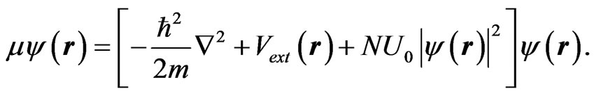
The three-dimensional form of the GPE can be written [11]
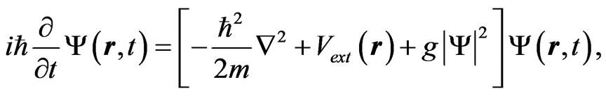 (1)
(1)
where  is Planck’s constant divided by
 ,
,  is the mass of the Boson,
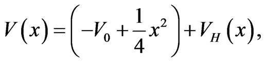
  is the confining trap potential, usually written as a sum of three harmonic potentials
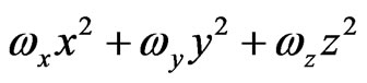 , and
, and  is a constant proportional to the number
  of particles in the trap times the scattering length
  of two of the Bosons. This constant can be written as [9]
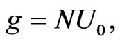 (2)
(2)
with
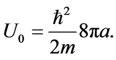 (3)
(3)
A stationary solution 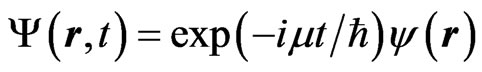 obeys [9]
 (4)
(4)
If one now assumes that  i.e., that the trap potential is spherically symmetric, makes a partial wave expansion of
 , and retains only the angular momentum
  part of the expansion,
 (5)
(5)
then  satisfies the radial Equation [9]
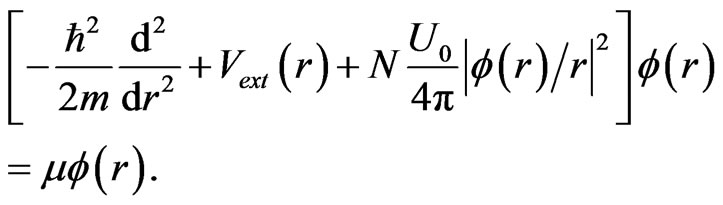 (6)
(6)
Here  describes the wave function of one of the particles, and since the probability of finding this particle is unity, i.e.,
  one finds, in view of Equation (5),
 (7)
(7)
The first, second, etc., iterations of  are denoted as
 , the corresponding Hartree potentials are denoted as
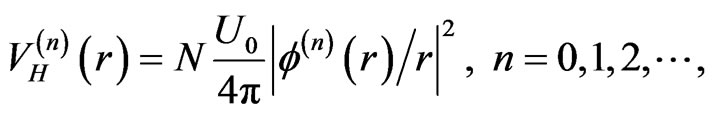 (8)
(8)
and the iterative equations are
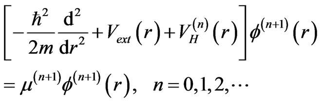 (9)
(9)
The functions  all go to zero at the origin of
 , decay to zero as gaussians as
  if
if  is assumed to be harmonic, and obey the normalization condition (7) for each iteration. For each fixed value of
 , the eigenfunctions
  and eigenvalues
  of Equation (9) are determined iteratively by a Hartree procedure described previously, both for bound states [39] as well as for Sturmian eigenvalues [40]. The feature that the function
  and the eigenvalue
  are determined simultaneously in each new iteration is what makes the present approach different from other iterative approaches. In summary, two nested iterations are performed: 1) One that finds the solutions of Equation (9) for each value of
 , and 2) The iterative progression from
  to
to  The latter proceeds non-monotonically, as seen in the numerical example given further on, and the first has been used successfully in several applications [41,42]. This double iteration procedure is different from the procedures cited above [9,10,12,13,20,46, 47]. Another difference from previous calculations is that the differential Equation (9) is transformed into a Lippmann-Schwinger integral equation, that is solved with the use of Green’s functions in configuration space [29, 39]. These functions require wave-numbers, rather than energies as input parameters. The calculations are done by means of a semi-spectral Chebyshev expansion method that gives a reliable accuracy [31-38].
2.1. Numerical Inputs
In order to solve Equations (8) and (9), two steps are required. First a set of physically reasonable values for the potentials have to be established, and subsequently a transformation of variables is made so as to render the equations more transparent, and all quantities become expressed in terms of new distance and energy units.
The atoms in the trap are assumed to have a mass  and the scattering length
  The confining trap potential is assumed to be harmonic
 (10)
(10)
and the value of the coefficient  is obtained by requiring that at a distance of
  from the center of the trap the value of
  with
with  This yields
  Next, both sides of Equation (6) are multiplied by
 , a new unit of distance
  is chosen
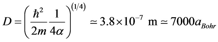 (11)
(11)
and by further multiplying by  Equation (9) is transformed into dimensionless units
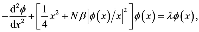 (12)
(12)
and the normalization Equation (7) is changed to
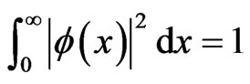 . (13)
Here
 (14)
(14)
 (15)
(15)
The energy unit  is thus
 . (16)
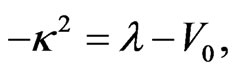
In order to solve Equation (12) numerically, a constant  is subtracted from both sides
with the result
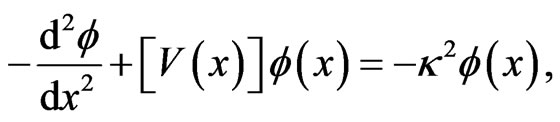 (17)
(17)
where
 (18)
(18)
 (19)
(19)
and where the dimensionless Hartree potential is given by
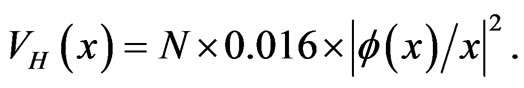 (20)
(20)
The effect of  is to move the bottom of the harmonic well to a negative energy, but
  still measures the eigenvalue energy above the bottom of the well. To this, thus moved harmonic potential, is added the Hartree potential
 , which is positive (repulsive) if the scattering length
  is positive. The advantage of having subtracted
  is that the wave number
  required as input to the Green’s function
  becomes purely imaginary,
  and thus the asymptotic value of
  decreases exponentially. However, since the potential
  continues to grow positively as
  increases, the asymptotic form of
  should decrease to zero like a Gaussian function. This behavior is indeed found to be the case in the numerical evaluations.
2.2. The Thomas-Fermi Approximation
This approximation to  is obtained by dropping the kinetic energy term from the GPE (4) or (6). As already noted previously [48,49], this approximation, denoted as
  gets better the larger the number
  of coherent atoms in the trap. However, since the function
  drops abruptly to zero at the outer edge of
 , it is difficult to incorporate this function into the numerical calculations [15,25]. This difficulty is overcome in the present investigation, by fitting to
  a smooth extension that decreases to zero exponentially, and subsequently using this fit for the start of the iterations for
 . The derivation of
  will be repeated here for completeness.
By discarding the second order derivative in Equation (12), one obtains
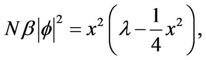 (21)
(21)
where the maximum value of  is
is  The value of
  is not known until one takes into account the normalization condition (13). The integrals can be done analytically for the case that the confining potential is harmonic, with the result
 (22)
(22)
The corresponding value of  is
is
 . (23)
A numerical example for the case that  is illustrated in Figure 1.
3. Results
As described in Section 2 the calculation consists of two nested iterations. For each Hartree potential  the corresponding eigenvalue
  and eigenfunction
  is calculated by a hybrid iterative method, implemented by means of a spectral Chebyshev expansion described in [39]. The resulting Hartree potential
 , given by
  is thus obtainedand so forth. Two different methods are used in order to initiate the procedure.
The first starts from the eigenfunction of the harmonic potential, in the absence of  the resulting function
 is fitted with a Woods-Saxon form, and after multiplication by
  the value of
  is obtained, and the process is repeated for subsequent iterations. Results with this method for the values
 are illustrated in Figure 2 for the ground state solutions. The convergence is oscillatory, and the gap between successive values of
  gradually decreases. The corresponding values of the ground state excitation energy are illustrated in Figure 3 by the points labelled as “H”, which also shows the oscillatory nature of the convergence. The first point, close to 1.4, corresponds to the excitation energy for the pure harmonic oscillator, which is smaller than the final excitation energy, close to 2.0. That increase is due to the repulsive nature of the Hartree potential.
The second method starts the iteration with a smoothed fit to the Thomas Fermi potential, as shown by the open circles in Figure 1. The corresponding excitation energies are displayed by the open circles in Figure
3. It is clear that the Thomas Fermi form for the Hartree potential provides a much better starting approximation for the iterations than the harmonic oscillator eigenfunction.
Not only the ground state of the GPE can be obtained with this iterative method starting from the fitted Thomas Fermi (TF) approximation to the Hartree potential, but with the same TF potential the higher excited states can also be obtained iteratively. The results for the ground, first and second excited states are displayed in Figure 4.
The excitation energies for the GPE lie above the values for the pure Harmonic potential well, confirming that the corresponding Hartree potentials are repulsive. It is interesting to note that for a larger value of the number  of coherent particles, the excitation energies are slightly lower. According to Equation (15) these energies are given in units of
 , Equation (16)
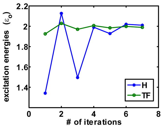
Figure 3. The ground state energies above the bottom of the attractive trap well, as a function of the number  of iterations. The iterations labeled “H” were started with the eigenfunction of the Harmonic well, while the ones labelled “TF” where started with a fit to the Thomas-Fermi approximation to the Hartree potential. The conditions are the same as in Figure 2, and the energies are given in terms of
 .
.
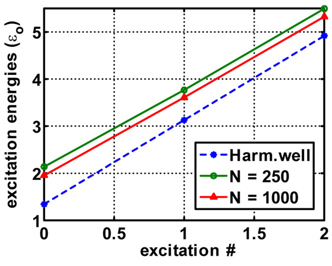
Figure 4. The final energies, in units of  of the ground, first and second excited states. The lowest set of points correspond to the harmonic well alone, and the other points are for the GP cases with N = 250 and 1000, respectively. The ground, first and second excited states are located on the x-axis at the points 0, 1, and 2, respectively.
The Hartree potentials, when added to the harmonic trap potential, are displayed in Figures 5 and 6 for the values of  and
and , respectively. The properties of the Hartree potentials can be inferred from these graphs: as
  increases, these potentials increase proportionally, but the functions
  do not change significantly.
Computational Details
The calculations are done with MATLAB on a desk PC using an Intel TM2 Quad, with a CPU Q 9950, a frequency of 2.83 GHz, and a RAM of 8 GB. For the case of  forty iterations take between 6 and 7 seconds. Table 1 of energy values for the ground and first excited states (in units of
  indicates the rate of convergence.
4. Summary and Conclusions
A method is presented of solving for the  partial wave function of the the Gross Pitaevskii nonlinear differential equation. A Hartree potential
  is used as a key vehicle for performing the iterations that converge for a low number of
  of atoms in the trap. This potential is defined as the wave-function squared times a factor proportional to the number
  of coherent atoms
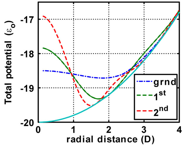
Figure 5. The sum of Harmonic and converged Hartree potentials for the ground, first and second BEC excited states, for N = 250, in units of .
.
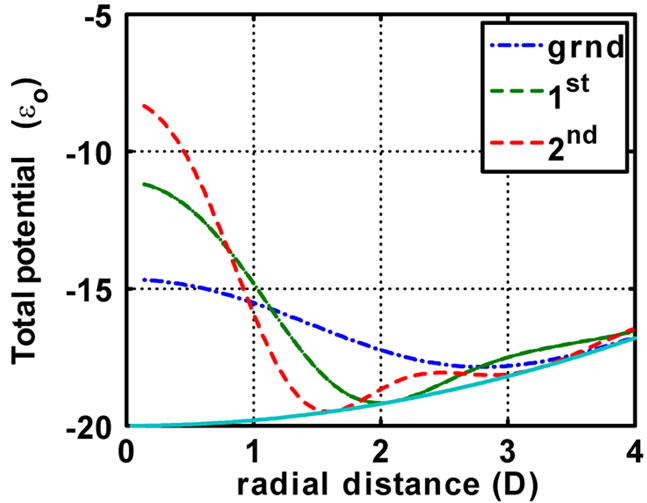
Figure 6. Same as Figure 5 for N = 1000 Please note the change in scale of the y-axis.
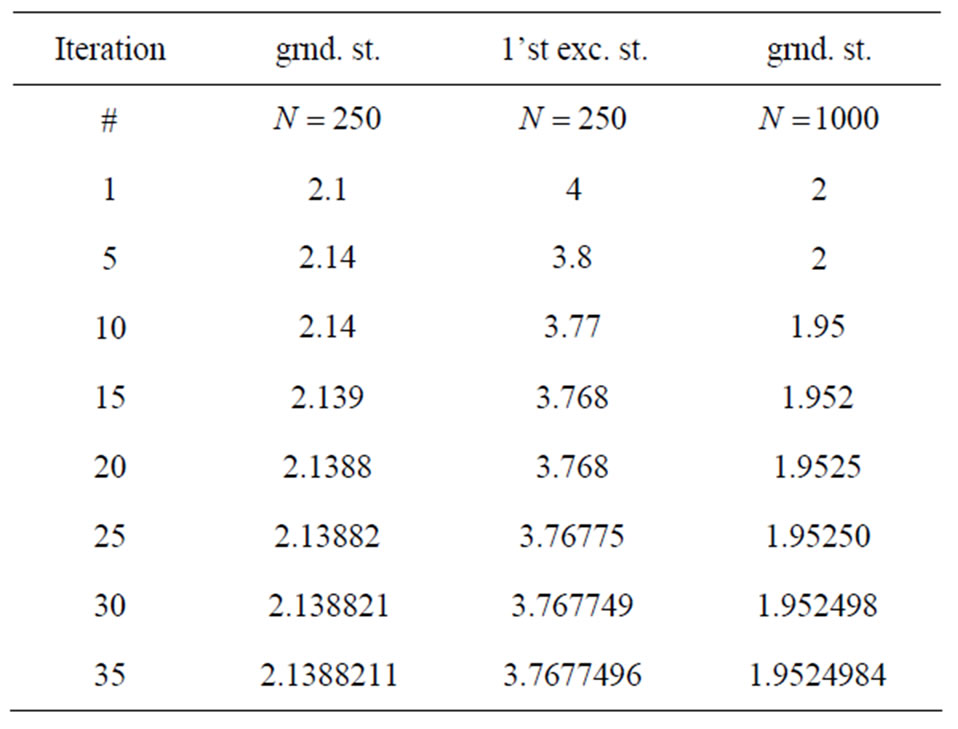
Table 1. Convergence of the excitation energies given in units described in the text.
and the (positive) scattering length. The parameters of the equation are determined from physical considerations. The Hartree potentials and binding energies are obtained for the ground, first and second excited states for  and
and  It is found that the start of the iterative process based on the Thomas-Fermi approximation to
  is more efficient than when the iterations are started from the eigenfunction of the harmonic well, as is shown in Figure 3. The iterations that lead from one
  to the next, as described in Equation (9), converge rather slowly. After each 5 iterations the stability of the excitation energy increases approximately by one significant figure, but the computational complexity is not excessive. The knowledge of
  is suggestive for future applications, such as for refining a mean-field potential for nucleons in a nucleus, once the Pauli exclusion principle for the nucleons is taken into account. This approach may lead to different nuclear mean field potentials for different shells.
NOTES