1. Introduction
The multi-point boundary value problems arising from applied mathematics and physics have received a great deal of attention in the literature (for instance, [1] -[4] and references therein). But, by so far, few results are about the existence of more than five solutions. To the author’s knowledge, there are very few papers concerned with the existence of countable positive solutions for multiple point BVPS (for instance, [5] and references therein). In [5] , the authors discussed the existence of countable positive solutions of n-point boundary value problems for a p-Laplace operator on the half-line. Directly inspired by [5] , in this paper, by using a fixed-point theorem, we study the existence of countable positive solutions of the following n-point boundary value problems.
 (1.1)
(1.1)
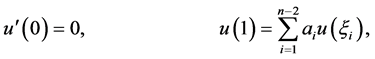 (1.2)
(1.2)
where ,
,  ,
,  ,
, .
.  and
and  has countable many singularities in
 .
.
This kind of problem arises in the study of a number of chemotherapy, population dynamics, ecology, industrial robotics and physics phenomena. Moreover, many problems in optimal control system, neural network (for example in BAM neural network) and information systems for computational science and engineering (especially in Internet-based computing) can be established as differential equation models with boundary condition (see, for instance, [6] and references therein).
At the end of this section, we state some definitions and lemmas which will be used in Section 2 and Section 3.
Definition 1.1 A map  is said to be a nonnegative, continuous, concave function on a cone
  of a real Banach space
 , if
, if  is continuous, and

for all  and
and .
.
Definition 1.2 Given a nonnegative continuous function  on a cone
 , for each
 , we define the set
Lemma 1.1 [7] Let  be a Banach space and
  be a cone in
 . Let
. Let , be three increasing, nonnegative and continuous functions on
 , satisfying for some
  and
and  such that
for all . Suppose that there exists a completely continuous operator
  and
and  such that 1)
 , for
, for .
.
2) , for
, for .
.
3) , and
, and , for
, for .
.
Then  has at least three fixed points
  such that

This paper is organized as follows: The preliminary lemmas are in Section 2. The main results are given in Section 3. Finally, in Section 4, we give an example to demonstrate our results.
2. The Preliminary Lemmas
In this paper, we will use the following space  and
and  is a Banach space with the norm
 . Let
. Let , we define a cone
  by
by
 .
.
For convenience, let us list some conditions.

 and on any subinterval of
  and when
  is bounded,
  is bounded on
 .
.
 There exists a sequence
  such that
 ,
,  ,
,  ,
,  , and
, and .
.
Lemma 2.1. Let ,
,  and
and  on
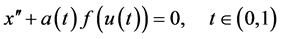
on , then the boundary value problem
 (2.1)
(2.1)
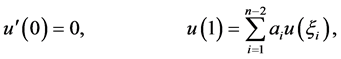 (2.2)
(2.2)
has a unique solution
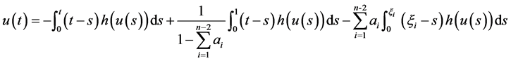
Proof. The proof is easy, so we omit it.
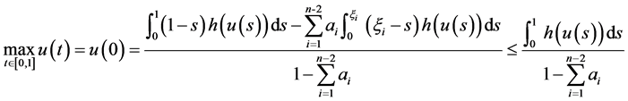
By , we know
  is decreasing and concave on
 . Then we have
 (2.3)
(2.3)
 (2.4)
(2.4)
From (2.3), (2.4) and the concavity of , we can easily get the following lemma.
Lemma 2.2. Let , if
, if  and
and , then the unique solution
  of (2.1)-(2.2) satisfies
  and
and , where
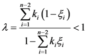 .
.
For , we define an operator
  by
by
 (2.5)
(2.5)
For , then
 , by
, by , we know
  is bounded on
 .
.
So there exists , such that
 . (2.6)
It is easy to see that  is decreasing and concave on
 . Then for
 , we have
 , that is
 . (2.7)
From , (2.3) and (2.6), we have
 (2.8)
(2.8)
From (2.7), (2.8), we can get the following lemma.
Lemma 2.3. Suppose  and
and  are satisfied. Then
  is bounded.
Lemma 2.4. Assume ,
, are satisfied, then
  is completely continuous.
Proof. From Lemma 2.2, we know  is bounded. If
  is a bounded subset of
 , then
  is uniformly bounded on
 .
.
For any ,
,  , without loss generality, we may assume
 , by (2.5), (2.6),
  , we have

uniformly as .
.
So  is equi-continuous on
 .
.
At last, by (2.5),  , the Lebesgue dominated convergence theorem and continuity of
 , we know
  is continuous. Then by the Arzela-Ascoli theorem, we can get that
  is completely continuous.
3. Main Results
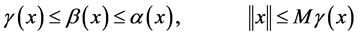
Let ,
,  and
and  be three nonnegative, decreasing and continuous functions with

Obviously, for  we have
 .
.
In the following, we let

Then it is easy to see .
.
The main result of this paper is as follows.
Theorem 3.1. Assume that  hold. Let
  be such that
 ,
,  be such that
  and
and
 .
. .
.
Furthermore for each natural number  we assume that
  satisfies:
 for all
 for all
 for all
 .
.
Then the BVP (1.1)-(1.2) has at least three infinite families of positive solutions
 with
with
 ,
,  ,
,  , for
, for .
.
Proof. From the definition of , (2.7) and Lemma 2.4, it is easy to see that
 , for
, for  is completely continuous.
Next we show all the conditions of Lemma 1.2 hold.
For any , it is easy to see
 . From Lemma 2.2, we have
 , so
, so  (3.1)
(3.1)
First, we choose , then we have
 . From
  and (3.1), we can get
 , for
, for . Then with
 , it implies that
 , for
, for .
.
So 
Therefore, the first condition of Lemma 1.2 satisfies.
Next, we select . Then
 , we have
 , for
, for .
.
Again from , and Lemma (2.2) we can get that
Then , for
, for . By
. By , we have
 , for
, for .
.
So, there has
This implies the second condition of Lemma 1.2 is satisfied.
Finally, we only need to show the third condition of Lemma 1.2 is also satisfied.
We select , for
, for . Obviously,
  , hence
  is nonempty.
 , we have
 . Also from
  and Lemma (2.4), we can get
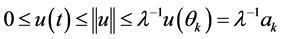 , for
, for . Then from
 , we have
 .
.
So .
.
Then all the conditions of Lemma 1.2 are satisfied. From Lemma 1.2, we get the conclusion in Theorem 3.1.
4. Example
Now we consider an example to illustrate our results.
Example 4.1. Consider the boundary value problem
 , (4.1)
 , (4.2)
Then the BVP (4.1)-(4.2) can be regarded as a BVP of the form (1.1)-(1.2) in . In this situation,
 .
.
Let ,
,  ,
, .
.
Consider the function , where


It is easy to know  satisfies.
Let ,
,  ,
,  be such that
 ,
,  be such that
 , and
, and 
 .
.
This with  implies that
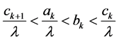 ,
,  ,
, .
.
Let 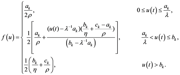
Obviously,  are satisfied, and it is easy to prove that
  is also satisfied. So all the conditions of Theorem 3.1 are satisfied, thus the BVP (4.1)-(4.2) has at least three infinite families of positive solutions
  satisfying
 ,
,  ,
,  , for
, for .
.
NOTES
*Corresponding author.