Transient Electro-Osmotic and Pressure Driven Flows through a Microannulus ()
1. Introduction
Microfluidic devices have become important due to their applications in medical science, biology, and analytical chemistry [1]. When an electrolyte comes in contact with a microchannel wall in which the fluid flows, the surface charge leads to the formation of an electric double layer (EDL) [2] and its ion density variation obeys the Boltzmann distribution [3]. When an electric field is applied tangentially along the charged surface, it will exert a Coulombic force on the ions within the EDL. The migration of the mobile ions will carry the adjacent and bulk liquid phase by viscosity, resulting in an electroosmotic flow (EOF). EOF is widely used in the fields of biology, chemistry and medicine.
Both theoretical and experimental investigations to steady EOF have been well studied in various microcapillaries geometric domains [4-12]. However, such steady electro-osmotic flows are likely to necessitate relatively larger voltages and field strengths, which might be rather undesirable in many practical situations. Recently, time periodic EOF has been attracting growing attention as an alternative mechanism of microfluidic transport. Dutta and Beskok [13] analytically investigated the time periodic EOF between two parallel plates, illustrating interesting similarities or dissimilarities with the Stokes second problem. A semi-analytical solution of periodical EOF in a rectangular microchannel was presented by Wang et al. [14] Chakraborty and Ray [15] investigated the mass flow-rate control through time periodic EOF in circular microchannels. Jian et al. [16] derived an analytical solution of velocity distribution for time periodic EOF in a cylindrical microannulus. Two limiting cases, i.e., the time periodical EOF approximately in parallel plate microchannel and circular microtube are discussed in their work. In addition, using separation of variable and Green function methods, Keh and Tseng [17] and Kang et al. [18] studied transient EOF in fine capillary and gave analytical expressions of electroosmotic velocity, respectively.
However, no one seems to have discussed, to the authors’ knowledge, transient mixed EOF/PDF through a microannulus. The purpose of current paper is to extend our recent work of time periodic EOF [16] to transient mixed EOF/PDF with a constant voltage in a cylindrical microannulus by the method of Laplace transform. The evolution of the EOF velocity at any time can be obtained.
2. Mathematical Formulation
2.1. Electrical Potential Distribution
The transient mixed EOF/PDF of incompressible Newtonian fluids through an annular region with inner radius  and outer radius R, the length of the channel is L, assumed to be much larger than the diameter, i.e.,
  is shown in Figure 1. The electrolyte fluid is acted upon by an axial (along z-direction) steady electric field of strength E0. The chemical interaction of electrolyte liquid and solid wall generates an EDL, a very thin charged liquid layer at the solid-liquid interface. A cylindrical coordinate system
  is adopted. In this theoretical model, the channel wall is assumed to be uniformly charged so that the electrical potential in the EDL varies in the r direction only and do not depend on θ. For a symmetric binary electrolyte solution, assuming the electrical potential ψ of the EDL is steady, and its distribution and the local volumetric net charge density
  are described by the Poisson-Boltzmann equations
 (1)
(1)
 (2)
(2)
here ε is the dielectric constant of the electrolyte liquid, n0 is the ion density of bulk liquid, zν is the valence, e0 is the electron charge, kb is the Boltzmann constant, and T is the absolute temperature. Substituting Equation (2) into Equation (1), the electrical potential in the annulus region can be expressed as
 (3)
(3)
which is subject to the following boundary conditions
 (a)
(a) (b)
(b)
Figure 1. (a) Sketch of transient electro-osmotic flow through a microannulus along z direction; (b) Cross section of the microannulus.
 , at
, at  (4a)
(4a)
 at
at  (4b)
(4b)
where the ςo is the outer capillary wall zeta potential and the ςi is the inner capillary wall zeta potential. For simplicity, the following dimension dimensionless groups are introduced
 (5)
(5)
Here κ is the Debye-Hückel parameter and 1/κ denotes the thickness of the EDL, and K is called the non-dimensional electrokinetic width. The dimensionless electrical potential Equation (3) and the corresponding boundary condition (4) can be written as
 (6)
(6)
 at
at  (7a)
(7a)
 at
at  (7b)
(7b)
Assuming the electrical potential is small enough, the Debye-Hückel linearization approximation can be used for the hyperbolic sine function appearing in the right hand side of Equation (6), which means physically that the electrical potential is small compared with the thermal energy of the charged species. Equation (6) can be simplified as
 (8)
(8)
Equation (8) is a modified Bessel equation, and its solution has the following form
 (9)
(9)
where I0 and K0 is the modified Bessel functions of first and second kinds of order zero, respectively. Substituting boundary conditions of Equation (7) into Equation (9), the constants of A1 and B1 can be determined as
 (10)
(10)
here  is defined as the ratio of the zeta potentials of the inner wall to the outer wall of the annulus. Substituting Equation (10) into Equation (9), the final electrical potential can be expressed as
 (11)
(11)
and the constants A and B are
 (12)
(12)
2.2. Velocity Distribution
In the presence of the applied electric field, the equation of the motion through the annulus due to electro-osmosis is given by the Navier-Stokes equation
 (13)
(13)
Here ρ is the fluid density,  is the axial velocity component, which is along with z-direction, μ is the fluid viscosity, p is pressure, and E0 is constant electric field of strength. In fact, we have assumed that the timedependent EOF does not affect the charge distribution in the Debye layer in Equation (13). Generally, the transient effect of EDL relaxation can be neglected because the time scale related to electro migration in the EDL is at least two orders smaller that the characteristic time associated with the evolution of the EOF [19]. The boundary conditions of Equation (13) are supposed no slip and can be written as
 at
at  (14a)
(14a)
 at
at  (14b)
(14b)
It is important to mention here that the boundary conditions at the walls may exhibit apparent slip behavior instead of following the classical no-slip conjecture. Such deviations, not being the focal point of concern in the present study, are not considered here. Introducing the following dimensionless groups:
 (15)
(15)
where  is the normalized pressure gradient applied along the channel axis.
Using Equations (2) and (8), for small zeta potential, the Equation (13) can be normalized as
 (16)
(16)
The normalized boundary conditions Equation (14) are
 at
at  (17a)
(17a)
 at
at  (17b)
(17b)
Let us employ the method of Laplace transform defined by
 (18)
(18)
If initial condition satisfies , then the transforms of Equations (16) and (17) give
 (19)
(19)
 at
at  (20a)
(20a)
 at
at  (20b)
(20b)
Substituting Equation (11) into Equation (19), we have
 (21)
(21)
Equation (21) is linear and inhomogeneous ordinary differential equation, and its solution can be expressed by the sum of a general solution  corresponding to homogeneous equation and a special solution
 (22)
(22)
The homogeneous solution of Equation (21) is written as
 (23)
(23)
here E and F are constants, which can be determined from boundary conditions of Equation (23). Considering the formation of the right hand side of Equation (21), the special solution can be expressed as
 (24)
(24)
here C and D are constants. Substituting Equation (24) into Equation (21) yields
 (25)
(25)
From Equation (8), we can obtain easily
 (26)
(26)
Substituting Equation (26) into Equation (25) and equalizing the coefficients in front of the modified Bessel functions I0 and K0 at the two sides of the equation yields
 (27)
(27)
Inserting Equations (23) and (24) into Equation (22), the solution of velocity  is
is
 (28)
(28)
Using boundary conditions of Equation (20), we can determine the constants E and F as
 (29)
(29)
 (30)
(30)
Now the analytical solution of Laplace transform of EOF velocity through a microannular can be determined by Equation (28) with related constants given by Equations (12), (27), (29) and (30). Then using the method of inverse Laplace transform defined by
 (31)
(31)
where  is a vertical line to the right of all singularities of
  in the complex s plane. Due to the complexity of the express of
 , the exact solution of the EOF velocity can not be obtained analytically. Therefore, the numerical computation must be performed by numerical inverse Laplace transform [20].
The analytical solution of Newtonian fluid velocity in the steady state can be expressed as
 (32)
(32)
where,

(33)
 (34)
(34)
3. Results and Discussions
In the previous section, dimensionless transient EOF velocity depend mainly on the electrokinetic width K, inner to outer radius ratio α, inner to outer zeta potential ratio β and the normalized pressure gradient Ω. In this section, we will discuss the influence of these parameters on the dimensionless transient EOF velocity.
For fixed α = 0.4, Figure 2 illustrates the variations of normalized EOF velocity at different time (0.02, 0.06, 0.12 and 0.20) with radius for different inner to outer zeta potential ratio β (−1, 0, 1 and 2). It can be seen from Figure 2 that for negative inner to outer zeta potential ratio β (see Figure 2(a)), the directions of the EOF velocity near EDL of two microannulus wall are inverse. However, for positive inner to outer zeta potential ratio β (see Figures 2(b)-(d)), the directions of the EOF velocity within the whole gap of the microannulus are uniform.
Larger β leads to larger velocity near the inner microannulus wall. The reason is that the electric force determined by electrical potential is mainly concentrated in the EDL, appreciable reductions in velocity are observed to occur outside the EDL. In addition, with the increase of time, the EOF velocity approaches gradually steady status. That is to say, further increase of the time will lead to invariable velocity profile.
For fixed β = 1, Figure 3 shows the variations of normalized EOF velocity at different time with radius for different inner to outer radius ratio α (0.2, 0.4, 0.6 and 0.8). Similarly, with the increase of time, the EOF velocity approaches gradually steady status. In addition, with the increase of inner to outer radius ratio α, the gap between the two walls of microannulus becomes small, thus the time needed to attain the steady status become small. The velocity profile changes from plug-like to parabolic-like shape.
For fixed α = 0.2, Figures 4(a)-(c) shows the variations of normalized EOF velocity at different time with different normalized pressure gradient . For a given dimensionless time, along with the dimensionless pressure gradient increased velocity amplitude section bigger. The reason is that dimensionless pressure gradient increases mean the driving force of pressure

Figure 2. Variations of normalized EOF velocity at different time with radius for different . (a) β = −1; (b) β = 0; (c) β = 1; (d) β = 2.
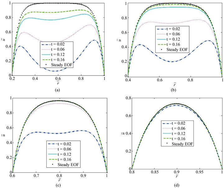
Figure 3. Variations of normalized EOF velocity at different time with radius for different . (a) α = 0.2; (b) α = 0.4; (c) α = 0.6; (d) α = 0.8.
increase. So the dimensionless velocity amplitude increases. In addition, with the increase of time, the EOF velocity approaches gradually steady status. Figure 4(d) depicts the flow of the fluids only under pressure-driven, i.e., no external electroosmotic flow, equivalent to Poiseuille flow.
Under the different dimensionless parameters, Figures 2-4 respectively compared the numerical solution with the analytical solution in steady state. As can be seen in the Figures 2-4, they are essentially coincident.
4. Conclusions
A semi-analytical solution of the transient mixed EOF/ PDF of Newtonian fluids through a microannulus under the Debye-Hückel approximation is presented in this work. The solution involves analytically solving the linearized Poisson-Boltzmann equation and Navier-Stokes equation. The results show that the velocity profiles depend greatly on the non-dimensional electrokinetic width K, the inner to outer radius ratio α, the inner to outer wall zeta potential ratio β and the normalized pressure gradient Ω. With the numerical computation of inverse Laplace transform, the following conclusions are drawn:
1) The inner to outer wall zeta potential ratio β determines the direction and magnitude of EOF velocity. Negative β leads to the inverse directions of the EOF velocity near EDL of two microannulus wall and vice versa. Larger β leads to larger velocity near the inner microannulus wall.
2) With the increase of inner to outer radius ratio α, the time needed to attain the steady status become less.
3) For a given dimensionless time, along with the dimensionless pressure gradient increased, velocity amplitude section becomes bigger.
The transient evolution of the velocity profiles provides a detail insight of the flow characteristic of this flow configuration.
5. Acknowledgements
Project supported by the National Natural Science Foundation of China (Grant Nos.:11062005, 11202092), Opening fund of State Key Laboratory of Nonlinear Mechanics, the program for young Talents of Science and Technology in Universities of Inner Mongolia Auton omous Region (Grant No. NJYT-13-A02), the Natural Science Foundation of Inner Mongolia (Grant Nos.: 2010BS0107, 2012MS0107), the research start up fund for excellent talents at Inner Mongolia University (Grant No.: Z20080211) and the support of Natural Science Key Fund of Inner Mongolia (Grant No: 2009ZD01), the Innovative programs funded projects of Postgraduate Education in Inner Mongolia Autonomous Region, and Inner Mongolia University of enhancing the comprehensive strength funding (Grant No. 1402020201).
NOTES