New Oscillation Results for Forced Second Order Differential Equations with Mixed Nonlinearities ()
1. Introduction
The oscillatory behavior of second order differential equations has a major role in the theory of differential equations. It has been shown that many real world problems can be modelled, in particular, by half linear differential equations which can be regarded as a natural generalization of linear differential equations [1- 14]. A considerable amount of research has also been done on quasi-linear [15-18] and nonlinear second order differential equations [19-23].
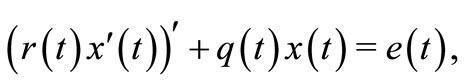
In this paper, we investigate the oscillatory behavior of second order forced differential equation with mixed nonlinearities.
 (1)
(1)
where ,
,  and
and  are real numbers,
 and
and  might alternate signs.
By a solution of Equation (1), we mean a function , where
  depends on the particular solution, which has the property that
  and satisfies Equation (1). We restrict our attention to the nontrivial solutions
  of Equation (1) only, i.e., to solutions
  such that
  for all
 . A nontrivial solution of (1) is oscillatory if it has arbitrarily large zeros, otherwise, it is called non-oscillatory. Equation (1) is said to be oscillatory if all its nontrivial solutions are oscillatory.
Equation (1) and its special cases such as the linear differential equation
 (2)
(2)
the half-linear differential equation
 (3)
(3)
and the quasi-linear differential equation
 (4)
(4)
have been extensively studied by numerous authors with different methods (see, for example, [1-5,15-19] and the references quoted therein).
In 1999, Wong [1] proved the following theorem by making use of the “oscillatory intervals” of e(t) and Leighton’s variational principle (see [10]) for (2).
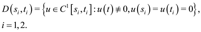
Theorem 1.1. Suppose that for any , there exist
  such that
 (5)
(5)
Denote
If there exist  such that
 (6)
(6)
then Equation (2) is oscillatory.
Afterwards, in 2002, the authors of [2] extended Wong’s results, using a similar method, to Equation (3) as follows.
Theorem 1.2. Suppose that for any , there exist
  such that (5) holds. Let

If there exist  and a positive, nondecreasing function
  such that
 (7)
(7)
for i = 1, 2, where , then (3) is oscillatory.
Later, in 2007, Zheng and Meng [16], considering a more general equation (4), improved the paper [2] and showed that the results obtained in [2] for Equation (3) can not be applied to the case . The main result of Zheng and Meng [16] is the following.
Theorem 1.3. Assume that for any , there exist
  such that (5) holds. Let

Suppose that there exist  and a positive, nondecreasing function
  such that
 (8)
(8)
for i =1, 2. Then Equation (4) is oscillatory, where
 (9)
(9)
with the convention that 
Also, in [2009], Zheng et al. [17] extended the results obtained for Equation (4) to Equation (1) as follows.
Theorem 1.4. Assume that for any , there exist
  such that
  for
for  and (5) holds. Let
 .
.
If there exist  and a positive function
  such that
 (10)
(10)
for i = 1, 2. Then Equation (1) is oscillatory, where
 (11)
(11)
with the convention that 
Recently, Shao [15] generalized the results of Zheng and Meng [16] by using the generalized variational principle due to Komkov [24] and gave the following result for Equation (4).
Theorem 1.5. Assume that, for any , there exist
  such that (1.5) holds. Let
 , and nonnegative functions
  satisfying
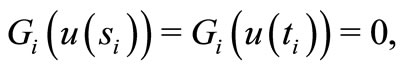
 are continuous and
for , i = 1, 2. If there exists a positive function
  such that
 (12)
(12)
for i = 1, 2, then Equation (4) is oscillatory, where  is the same as (9).
Motivated by the above theorems we propose some new oscillation results by employing the generalized variational principle and Riccati technique for Equation (1). Our results extend and generalize some known results in the literature. We now state our main results and several remarks.
2. New Oscillation Results
In order to prove our results we use the following wellknown inequality which is presented by Hardy et al. [25].
Lemma 2.1. (see [25]). If  and
and  are nonnegative, then
 (13)
(13)
where equality holds if and only if 
Theorem 2.1. Assume that, for any , there exist
  such that
 for
for  and (5)
holds. Let  and nonnegative functions
 satisfying

are continuous and

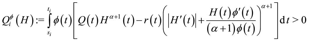
for , i = 1, 2. If there exists a positive function
  such that
 (14)
(14)
for i =1, 2, then Equation (1) is oscillatory, where  is the same as (11).
Proof. Suppose that  is a nonoscillatory solution of Equation (1). Then, there exists a
  such that
  for all
 . Without loss of generality, we may assume that
  for all
 . We introduce the Ricccati transformation
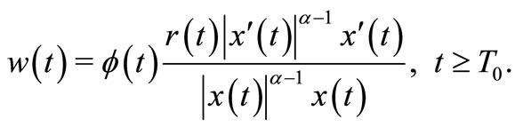 (15)
(15)
Differentiating (15) and using (1), we obtain, for all ,
,
 (16)
(16)
By the assumption, we can choose  so that
  on the interval
  with
with . As in [18], for given
 , set
, set

It is easy to verify that

So  obtains its minimum on
  and
and
 (17)
(17)
Then, by using (17) in (16), we get
 (18)
(18)
Multiplying  through (18) and integrating over
 , we have
 (19)
(19)
By integration by parts and using the fact that  we have
 (20)
(20)
In view of (19) and (20), we conclude that
 (21)
(21)
Let

According to Lemma 2.1, we obtain for 

Therefore, (21) yields

which contradicts the assumption (14) for .
.
When  is a negative solution for
 , we may employ the fact that
  on
on  to reach a similar contradiction. Therefore, any solution
  can be neither eventually positive nor eventually negative. Hence, any solution is oscillatory. This completes the proof of Theorem 2.1.
If  and
and , then Equation (1) reduces to Equation (4). Thus by Theorem 2.1, we have the following oscillation result:
Corollary 2.1. Assume that, for any , there exist
  such that (5) holds. Let
 , and nonnegative functions
  satisfying
 are continuous and
for  for i =1, 2. If there exists a positive function
  such that
 (22)
(22)
for i = 1, 2, then Equation (4) is oscillatory, where  is the same as (9).
Remark 1. Corollary 2.1 shows that Theorem 2.1 is a generalization of Theorem 1.5.
Remark 2. Let  in Corollary 2.1, then our main Theorem 2.1 reduces to Theorem 1.3.
Remark 3. If we choose  in Theorem 2.1, then we obtain Theorem 1.4.
Remark 4. If we choose  and
and  in Theorem 2.1, then we obtain Corollary 2.3 of Paper [17].
Remark 5. If we choose  and
and  in Corollary 2.1, then we obtain Corollary 2.3 of paper [16].
Remark 6. Let

and  in Theorem 2.1, then Theorem 2.1 is a generalization of Theorem 1.1.
Remark 7. Let  If we choose
  in Theorem 2.1, then Theorem 2.1 improves Theorem 1.2, since the positive constant
  in Theorem 2.1 can be chosen as any number lying in
 .
.
Remark 8. If the condition (5) in Theorem 2.1 and Corollary 2.1 is replaced by

then the results given in this paper are still valid.
3. Examples
Example 3.1. Consider
 (23)
(23)
for , where
  are constants. Let
and , so
, so . The zeros of forcing term
  are
are . For any
 , we choose
  sufficiently large so that
 ,
,
 and
and  Letting
 (it is easy to verify that
  for
for ),
),  then we obtain

and

Therefore, Equation (14) is satisfied for i = 1 provided that 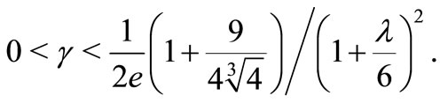 In a similar way, for
  and
and , we choose
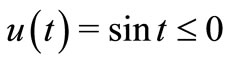 ,
,  (it is easy to verify that
  for
for ) so that that (14) is valid for i = 2. Thus (23) is oscillatory for

by Theorem 2.1.
Example 3.2. Consider the following forced quasilinear differential equation
 (24)
(24)
for , where
  are constants. Let
and , so
, so  The zeros of forcing term
  are
are . For any
we choose n sufficiently large so that  ,
,  and
and  Letting

 ,
,  then we obtain

and

Therefore, Equation (14) is satisfied for i = 1 provided that , where
In a similar way, for  and
and  , we choose
 ,
,  so that (14) is valid for i = 2. Thus (24) is oscillatory for
  by Theorem 2.1.
4. Conclusion
The oscillatory behavior of many different kinds of differential equations has been investigated and a great deal of results has been obtained in the literature. In this article, we generalized the results obtained in [16,17] and extended the results of Shao [15] by using the generalized variational principle and Riccati tecnique. In a similar way, the results obtained for Equation (1) can be extended to a more general class of differential equations.
5. Acknowledgements
The authors would like to express sincere thanks to the anonymous referee for her/his invauable corrections, comments and suggestions on the paper.