Hybrid Extragradient-Type Methods for Finding a Common Solution of an Equilibrium Problem and a Family of Strict Pseudo-Contraction Mappings ()
1. Introduction
Let  be a real Hilbert space endowed with an inner product
  and a norm
  associated with this inner product, respectively. Let C be a nonempty closed convex subset of
 , and f be a bifunction from C × C to R such that f(x, x) = 0 for all
 . An equilibrium problem in the sense of Blum and Oettli [1] is stated as follows:
 (1)
(1)
Problem of the form (1) on one hand covers many important problems in optimization as well as in nonlinear analysis such as (generalized) variational inequality, nonlinear complementary problem, nonlinear optimization problem, just to name a few. On the other hand, it is rather convenient for reformulating many practical problems in economic, transportation and engineering (see [1,2] and the references quoted therein).
The existence of solution and its characterizations can be found, for example, in [3], while the methods for solving problem (1) have been developed by many researchers [4-8].
Alternatively, the problem of finding a common fixed point element of a finite family of self-mappings
 (p ≥ 1)
is expressed as follows:
 (2)
(2)
where Fix(Si, C) is the set of the fixed points of the mapping Si (i = 1, ···, p).
Problem of finding a fixed point of a mapping or a family of mappings is a classical problem in nonlinear analysis. The theory and solution methods of this problem can be found in many research papers and mono-graphs (see [9]).
Let us denote by Sol(f, C) and
the solution sets of the equilibrium problem (1) and the fixed-point problem (2), respectively. Our aim in this paper is to address to the problem of finding a common solution of two problems (1) and (2). Typically, this problem is stated as follows:
 (3)
(3)
Our motivation originates from the following observations. Problem (3) can be on one hand considered as an extension of problem (1) by setting Si = I for all i = 1, ···, p, the identity mapping. On the other hand it is significant in many practical problems. Since the equilibrium problems have found many applications in economic, transportation and engineering, in some practical problems it may happen that the feasible set of those problems result as a fixed point solution set of one or many fixed point problems. In this case, the obtained problem can be reformulated in the form of (3). An important special case of problem (3) is that
and this problem is reduced to finding a common element of the solution set of variational inequalities and the solution set of a fixed point problem (see [10-12]).
In this paper, we propose a new hybrid iterative-based method for solving problem (3). This method can be considered as an improvement of the viscosity approximation method in [11] and iterative methods in [13]. The idea of the algorithm is to combine the extragradient-type methods proposed in [14] and a fixed point iteration method. Then, the algorithm is modified by projecting on a suitable convex set to obtain a new variant which possesses a better convergence property.
The rest of the paper is organized as follows. Section 2 recalls some concepts and results in equilibrium problems and fixed point problems that will be used in the sequel. Section 3 presents two algorithms for solving problem (3) and some discussion on implementation. Section 4 investigates the convergence of the algorithms presented in Section 3 as the main results of our paper.
2. Preliminaries
Associated with the equilibrium problem (1), the following definition is common used as an essential concept (see [3]).
Definition 2.1. Let C be a nonempty closed convex subset of a real Hilbert space . A bifunction f: C × C → R is said to be
1) Monotone on C if  for all x and y in C;
2) Pseudo-monotone on C if  implies
  for all x, y in C;
3) Lipschitz-type continuous on C with two Lipschitz constants c1 > 0 and c2 > 0 if
 (4)
(4)
It is clear that every monotone bifunction f is pseudo-monotone. Note that the Lipschitz continuous condition (4) was first introduced by Mastroeni in [7].
The concept of strict pseudo-contraction is considered in [15], which defined as follows.
Definition 2.2. Let C be a nonempty closed convex subset of a real Hilbert space . A mapping S: C → C is said to be a strict pseudo-contraction if there exists a constant 0 ≤ L < 1 such that
 (5)
(5)
where I is the identity mapping on . If L = 0 then S is called non-expansive on C.
The following proposition lists some useful properties of a strict pseudo-contraction mapping.
Proposition 2.3. [15] Let C be a nonempty closed convex subset of a real Hilbert space , S: C → C be an L-strict pseudo-contraction and for each i = 1, ···, p, Si: C → C is a Li -strict pseudo-contraction for some 0 ≤ Li < 1. Then:
1) S satisfies the following Lipschitz condition:
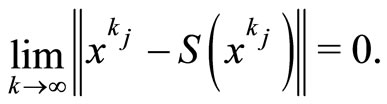
2) I − S is demiclosed at 0. That is, if the sequence {xk} contains in C such that  and
and  then
then ;
;
3) The set of fixed points Fix(S) is closed and convex;
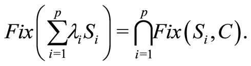
4) If  (i = 1, ···, p)
and 
then 
is a  -strict pseudo-contraction with
 ;
;
5) If  is chosen as in (d) and
  has a common fixed point then:
Before presenting our main contribution, let us briefly look at the recently literature related to the methods for solving problem (3). In [11], S. Takahashi and W. Takahashi proposed an iterative scheme under the name viscosity approximation methods for finding a common element of set of solutions of (1) and the set of fixed points of non-expansive mapping S in a real Hilbert space . This method generated an iteration sequence {xk} starting from a given initial point
  and computed xk + 1 as
 (6)
(6)
where g is a contraction of  into itself, the sequences of parameters {rk} and {αk} were chosen appropriately. Under certain choice of {αk} and {rk}, the authors showed that two iterative sequences {xk} and {uk} converged strongly to
 where PrC denotes the projection onto C.
Alternatively, the problem of finding a common fixed point of a finite sequence of mappings has been studied by many researchers. For instance, Marino and Xu in [7] proposed an iterative algorithm for finding a common fixed point of p strict pseudo-contraction mapping Si (i = 1, ···, p). The method computed a sequence {xk} starting from  and taking:
 (7)
(7)
where the sequence of parameters {λk} was chosen in a specific way to ensure the convergence of the iterative sequence {xk}. The authors showed that the sequence {xk} converged weakly to the same point
 .
.
Recently, Chen et al. in [13] proposed a new iterative scheme for finding a common element of the set of common fixed points of a strict pseudo-contraction sequence  and the set of solutions of the equilibrium problem (1) in a real Hilbert space
 . This method is briefly described as follows. Given a starting point
  and generates three iterative sequences {xk}, {yk} and {zk} using the following scheme:
 (8)
(8)
Here, two sequences {αk} and {rk} are given as control parameters. Under certain conditions imposed on {αk} and {rk}, the authors showed that the sequences {xk}, {yk} and {zk} converged strongly to the same point x* such that
 where S is a mapping of C into itself defined by
for all .
.
The solution methods for finding a common element of the set of solutions of (1) and
in a real Hilbert space have been recently studied in many research papers (see [8,12,16-23]). Throughout those papers, there are two essential assumptions on the function f have been used: monotonicity and Lipschitztype continuity.
In this paper, we continue studying problem (3) by proposing a new iterative-based algorithm for finding a solution of (3). The essential assumptions that will be used in our development includes: pseudo-monotonicity and Lipschitz-type continuity of the bifunction f and the strict pseudo-contraction of Si (i = 1, ···, p). The algorithm is then modified to obtain a new variant which has a better convergence property.
3. New Hybrid Extragradient Algorithms
In this section we present two algorithms for finding a solution of problem (3). Before presenting algorithmic schemes, we recall the following assumptions that will be used to prove the convergence of the algorithms.
Assumption 3.1. The bifunction f satisfies the following conditions:
1) f is pseudo-monotone and continuous on C;
2) f is Lipschitz-type continuous on C;
3) For each ,
,  is convex and subdifferentiable on C.
Assumption 3.2. For each i = 1, ···, p, Si is Li-strict pseudo-contraction for some 0 ≤ Li < 1.
Assumption 3.3. The solution set of (3) is nonempty, i.e.
 (9)
(9)
Note that if
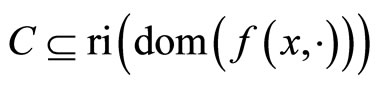
where
is the set of relative interior points of the domain of , then Assumption 3.1 3) is automatically satisfied. The first algorithm is now described as follows.
Algorithm 3.4
Initialization: Given a tolerance ε > 0. Choose three positive sequences {λk}, {λk, i} and {αk} satisfy the conditions:
 (10)
(10)
Find an initial point . Set
. Set .
.
Iteration k: Perform the two steps below:
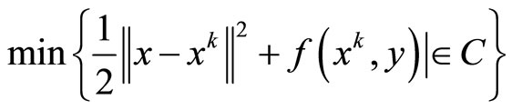
Step 1: Solve two strongly convex programs:
 (11)
(11)
Step 2: Set
 .
.
Set  and go back to Step 1.
The main task of Algorithm 3.4 is to solve two strongly convex programming problems at Step 1. Since these problems are strongly convex and C is nonempty, they are uniquely solvable. To terminal the algorithm, we can use the condition on step size by checking  for a given tolerance ε > 0. Step 1 of Algorithm 3.4 is known as an extragradient-type step for solving equilibrium problem (1) proposed in [14]. Step 2 is indeed the iteration (7) of the iterative method proposed in [24].
As we will see in the next section, Algorithm 3.4 generates a sequence {xk} that converges weakly to a solution x* of (3). Recently, a modification of Mann’s algorithm for finding a common element of p strict pseudo-contractions was proposed [15]. The authors proved that this algorithm converged strongly to a common fixed point of the p strict pseudo-contractions. In the next algorithm, we extended the algorithm in [15] for finding a common solution of the set of common fixed points of p strict pseudo-contractions and the equilibrium problems to obtain a strongly convergence algorithm. This algorithm is similar to the iterative scheme (8), where an augmented step will be added to Algorithm 3.4 and obtain a new variant of Algorithm 3.4.
For a given closed, convex set X in  and
and , PrX(x) denotes the projection of x onto X. The algorithm is described as follows.
Algorithm 3.5
Initialization: Given a tolerance ε > 0. Choose positive sequences {λk}, {λk, i} and {αk} satisfy the conditions (10) and the following addition condition:
 (12)
(12)
Find an initial point . Set
. Set .
.
Iteration k: Perform the three steps below:
Step 1: Solve two strongly convex programs:
 (13)
(13)
Step 2: Set
 .
.
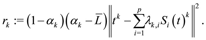
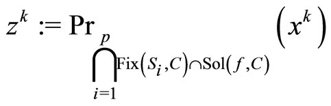
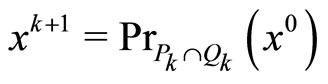
Step 3: Compute
 (14)
(14)
where
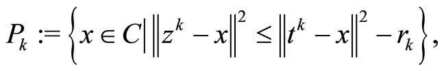
 (15)
(15)
Set  and go back to Step 1.
The augmented step needed in Algorithm 3.5 is a simple projection on the intersect of two half-planes. The projection is cheap to compute in implementation.
4. The Convergence of the Algorithms
This section investigates the convergence of the algorithms 3.4 and 3.5. For this purpose, let us recall the following technical lemmas which will be used in the sequel.
Lemma 4.1 [25]. Let C be a nonempty closed convex subset of a real Hilbert space . Suppose that, for all
 , the sequence {xk} satisfies
Then the sequence 
converges strongly to some .
.
Using the well-known necessary and sufficient condition for optimality in convex programming, we have the following result.
Lemma 4.2 [2]. Let C be a nonempty closed convex subset of a real Hilbert space  and g: C → R be subdifferentiable on C. Then x* is a solution to the following convex problem
if and only if
 where
where  denotes the subdifferential of g and
  is the (outward) normal cone of C at
 .
.
The next lemma is regarded to the property of a projection mapping.
Lemma 4.3 [9]. Let C be a nonempty closed convex subset of a real Hilbert space  and
and . Let the sequence {xk} be bounded such that every weakly cluster point
  of {xk} belongs to C and
Then xk converges strongly to PrC(x0) as k → ∞.
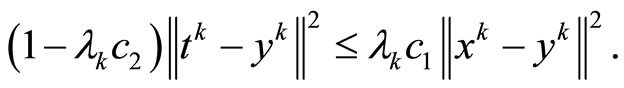
Lemma 4.4 (see [14], Lemma 3.1). Let C be a nonempty closed convex subset of a real Hilbert space . Let
. Let  be a pseudomonotone, Lipschitztype continuous bifunction with constants c1 > 0 and c2 > 0. For each
 , let
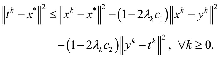
, let  be convex and subdifferentiable on C. Suppose that the sequences {xk}, {yk}, {tk} generated by Scheme (13) and
 . Then
Now, we prove the main convergence theorem.
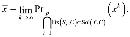
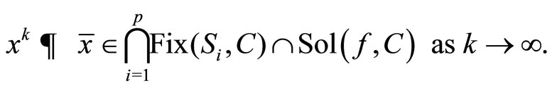
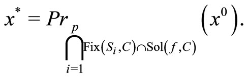
Theorem 4.5. Suppose that Assumptions 3.1-3.3 are satisfied. Then the sequences {xk}, {yk} and {zk} generated by Algorithm 3.4 converge weakly to the same point
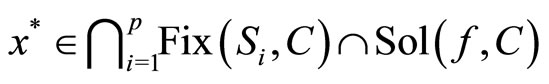
where
 (16)
(16)
Proof. The proof of this theorem is divided into several steps.
Step 1. We claim that
Indeed, for each k ≥ 1, we denote by
 .
.
By statement 4) of Proposition 2.3, we see that  is a
is a  -strict pseudo-contraction on C and then
 .
.
Now, we suppose that
 .
.
Then, using Lemma 4.4 and the relation
 for all
  and
and , we have
 (17)
(17)
 (18)
(18)
 (19)
(19)
Therefore, there exists
 .
.
It follows from (18) that
 .
.
So we have
Using this and
we have
 .
.
Similarly, we also have
 .
.
Then, since
we also have
 .
.
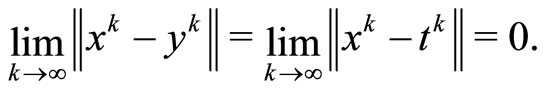
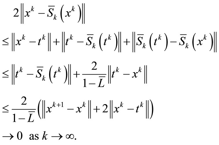
Step 2. We show that
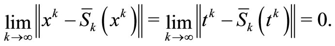
It follows from (17) that
Combining this and Lemma 4.4, we get
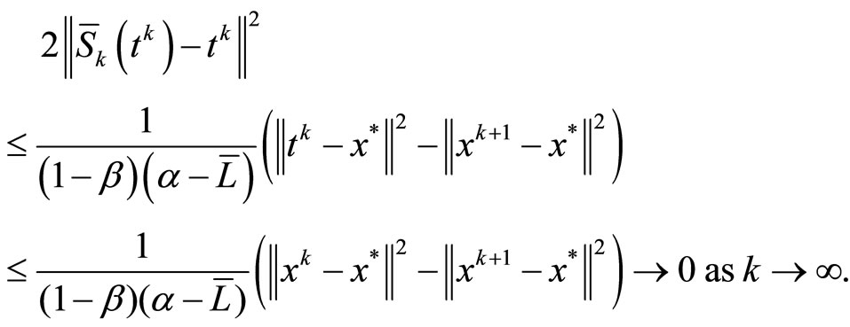
Then, using (a) of Proposition 2.3 and Step 2, we obtain
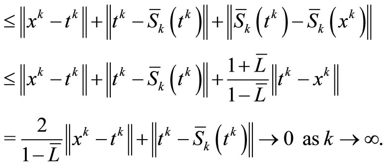
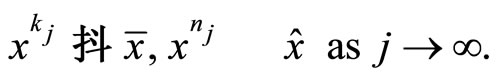
In Step 3 and Step 4 of this theorem, we will consider weakly clusters of {xk}. It follows from (19) that the sequence {xk} is bounded and hence there exists a subsequence  converges weakly to
  as j → ∞.
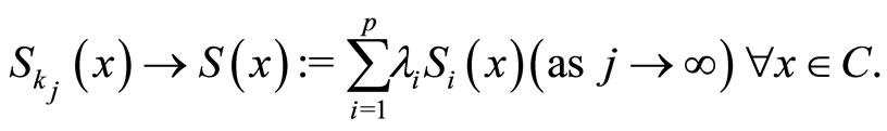
Step 3. We show that
 .
.
Indeed, for each i = 1, ···, p, we suppose that  converges
  as j → ∞ such that
 .
.
Then we have
Since  from Step 2 and
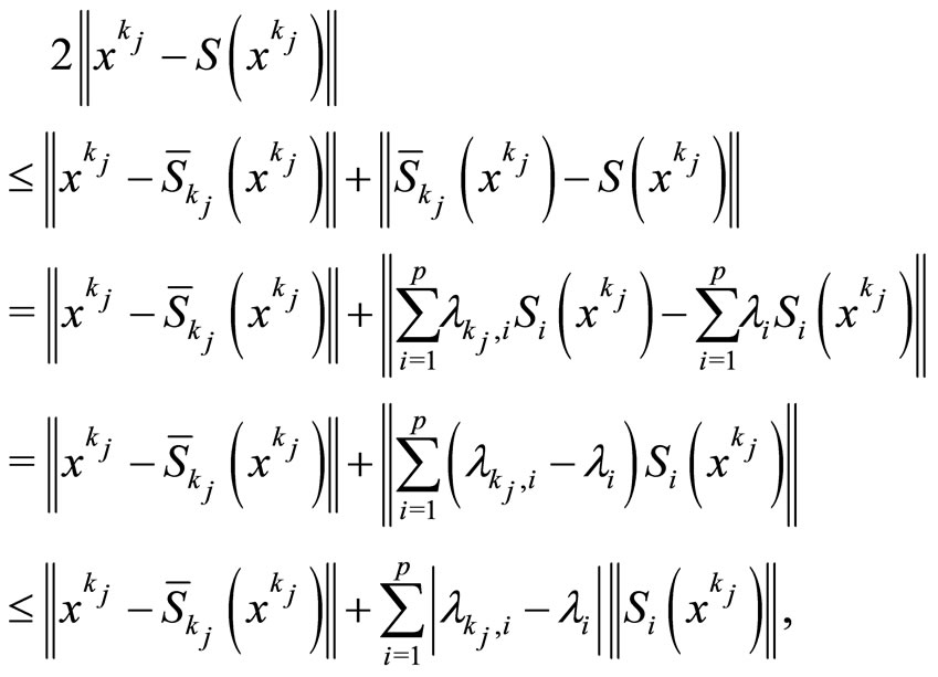
we obtain that
By 2) of Proposition 2.3, we have
 .
.
Then, it implies from 5) of Proposition 2.3 that
 .
.
Step 4. When  as j → ∞, we show that
  Indeed, since yk is the unique strongly convex problem
and Lemma 4.2, we have
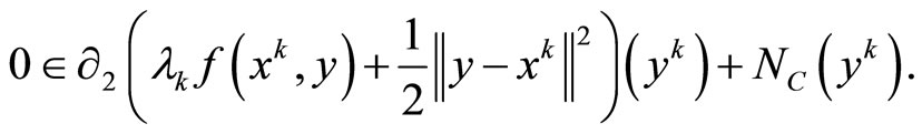
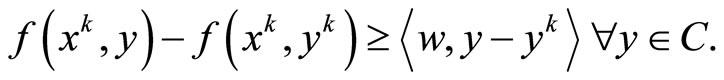
This follows that
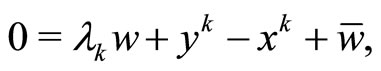
where  and
and . By the definition of the normal cone NC we imply that
 (20)
(20)
On the other hand, since  is subdifferentiable on C, by the well known Moreau-Rockafellar theorem, there exists
such that
Combining this with (20), we have

Hence
Then, using
Step 2,  as j → ∞ and continuity of f, we have
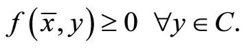
This means that .
.
Step 5. We claim that the sequences {xk}, {yk} and {tk} convergence weakly to  as k → ∞, where
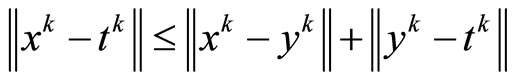
Indeed, since {xk} is bounded, we suppose that there exists two sequences  and
and  such that
By Step 3 and Step 4, we have
 .
.
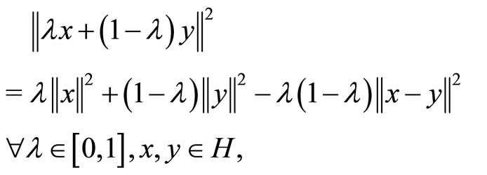
Then, using 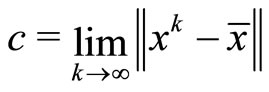
and the following equality (see [7])
where  as k → ∞, we have
Hence, we have . This implies that
Then, it follows from Step 2 that  as k → ∞.
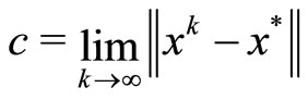
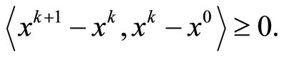
Now, we suppose that
and  as k → ∞. By the definition of PrC(·), we have
 (21)
(21)
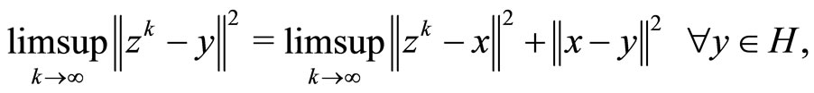
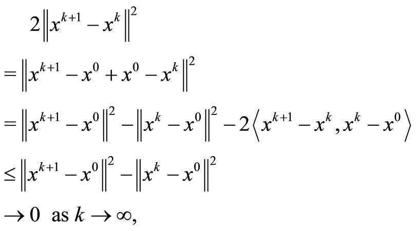
It follows from Step 1 that
Then, by Lemma 4.1, we have
 (22)
(22)
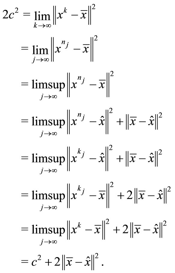
Pass the limit in (21) and combining this with (22), we have
This means that  and
and
It follows from Step 2 that the sequences {xk}, {yk} and {tk} converge weakly to  as k → ∞, where
The proof is completed.
The next theorem proves the strong convergence of Algorithm 3.5.
Theorem 4.6. Suppose that Assumptions 3.1-3.3 are satisfied. Then the sequences {xk} and {yk} generated by Algorithm 3.5 converge strongly to the same point x*
where 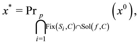
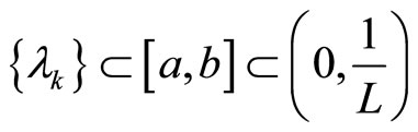
provided  .
.
Proof. We also divide the proof of this theorem into several steps.
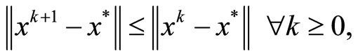
Step 1. We claim that
Indeed, for each
 it implies from (17) that
where
 .
.
This means that  and hence
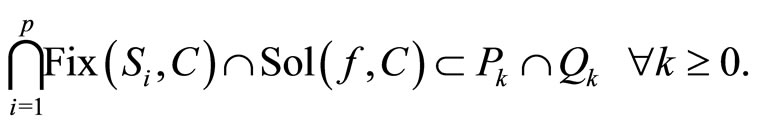
for all k ≥ 1. We prove
 (23)
(23)
by induction. For k = 0, we have
 .
.
As 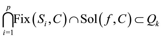
by the induction assumption and hence
 .
.
Since
we have
 .
.
Thus
By the definition of Qk + 1, we have
 .
.
Hence (23) holds for all k ≥ 0.
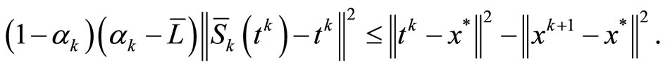
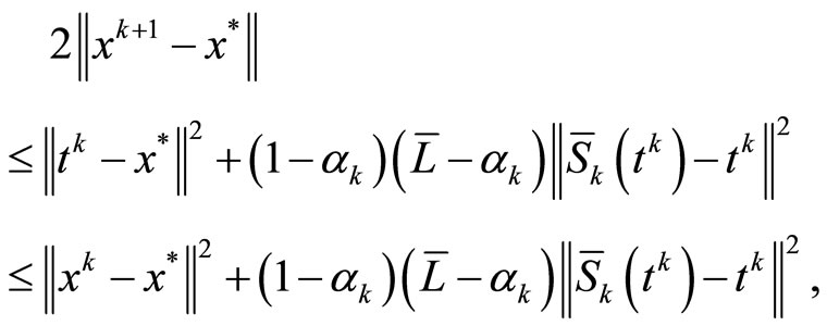
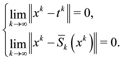
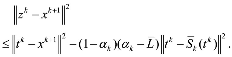
Step 2. We show that
Indeed, from 
it follows , i.e.,
Then, we have
the last claim holds by Step 1 of Theorem 4.5. From
 it follows that
 , i.e.
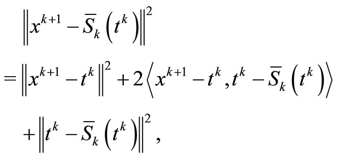
Using this and the following equality
we obtain
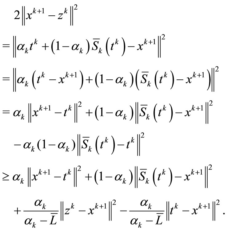
Hence
Combining this and
we have
 (24)
(24)
Since  is subdifferentiable on C, by the well known Moreau-Rockafellar theorem, there exists
  such that
With t = x*, this inequality becomes
 (25)
(25)
By the definition of the normal cone NC we have, from the latter inequality, that
 (26)
(26)
With t = yk, we have

Combining f(x, x) = 0 for all , the last inequality and the definition of w,
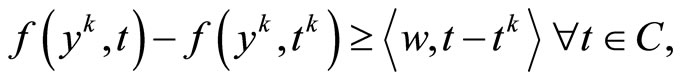
we have
 (27)
(27)
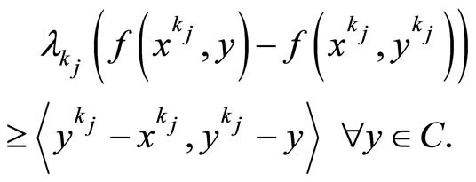
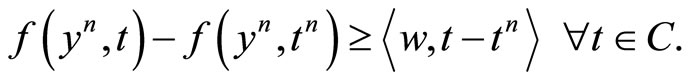
Since yn is the unique solution to the strongly convex problem
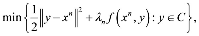
we have
 (28)
(28)
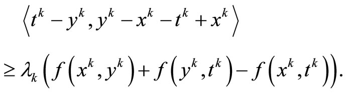
Substituting , we obtain
 (29)
(29)
From (29), it follows
 (30)
(30)
Adding two inequalities (27) and (30), we obtain
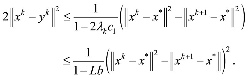
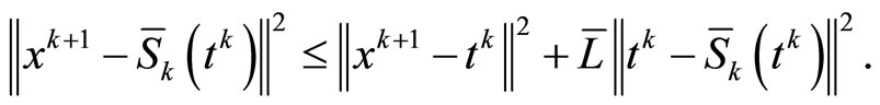
Then, since f is Lipschitz-type continuous on C, we have
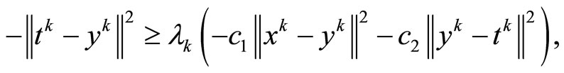
which follows that
From  it follows that
 .
.
Then, we have
 (31)
(31)
Since (24), (31) and  is Lipschitz continuous, we have
Step 3. We show that the sequence {xk} converges strongly to x*, where
Indeed, as in Step 4 and Step 5 of the proof of Theorem 4.5, we can claim that for every weakly cluster point  of the sequence {xk} satisfies
 .
.
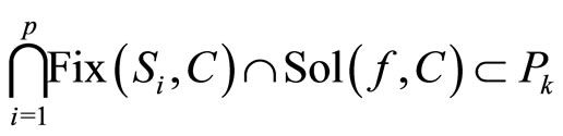
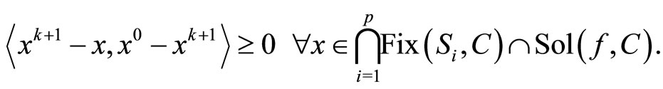
On the other hand, using the definition of Qk, we have
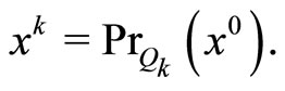
Combining this with Step 1, we obtain

With x = x*, we have
By Lemma 4.3, we claim that the sequence {xk} converges strongly to x* as k → ∞, where
 .
.
Hence, we also have yk → x* as k → ∞.
5. Acknowledgements
The work of the first author was supported by the Vietnam National Foundation for Science Technology Development (NAFOSTED), code 101.02-2011.07.