1. Introduction
In the recent literature there is a growing interest to solve integro-differential equations. The reader is referred to [1-3] for an overview of the recent work in this area. In the beginning of the 1980’s, Adomian [4-7] proposed a new and fruitful method (so-called the Adomian decomposition method) for solving linear and nonlinear (algebraic, differential, partial differential, integral, etc.) equations. It has been shown that this method yields a rapid convergence of the solutions series to linear and nonlinear deterministic and stochastic equations. The main objective of this work is to use the Combined Laplace Transform-Adomian Decomposition Method (CLT-ADM) in solving the nth-order integro-differential equations.
Let us consider the general functional equation
 (1.1)
(1.1)
where  is a nonlinear operator,
  is a known function, and we are seeking the solution y satisfying (1.1). We assume that for every
  Equation (1.1) has one and only one solution.
The Adomian’s technique consists of approximating the solution of (1.1) as an infinite series
 (1.2)
(1.2)
and decomposing the nonlinear operator  as
as
 (1.3)
(1.3)
where  are polynomials (called Adomian polynomials) of
  [4-7] given by

The proofs of the convergence of the series  and
and  are given in [6,8-12]. Substituting (1.2) and
(1.3) into (1.1) yields

Thus, we can identify

Thus all components of  can be calculated once the
  are given. We then define the n-terms approximant to the solution
  by
by  with
with

2. General nth-Order Integro-Differential Equations
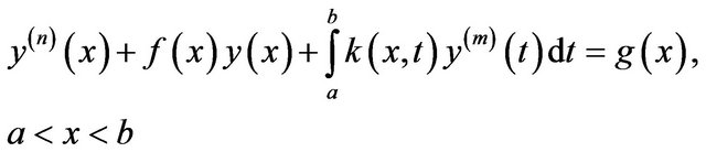
Let us consider the general nth-order integro-differential equations of the type [1,2]:
 (2.1)
(2.1)
with initial conditions

where  are real constants,
  and
and  are integers and
 . In Equation (2.1) the functions
  and the kernel
  are given real-valued functions, and
  is the solution to be determined. We assume that Equation (2.1) has the unique solution.
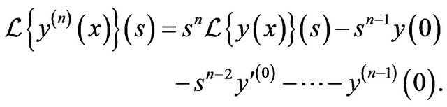
To solve the general nth-order integro-differential Equation (2.1) using, the Laplace transform method, we recall that the Laplace transforms of the derivatives of  are defined by
Applying the Laplace transform  to both sides of (2.1) and taking into account the fact that the convolution theorem for Laplace transform [13,14] gives:

This can be reduced to
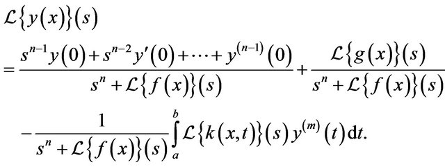 (2.2)
(2.2)
Substituting (1.2) into (2.2) leads to

The Adomian decomposition method presents the recursive relation
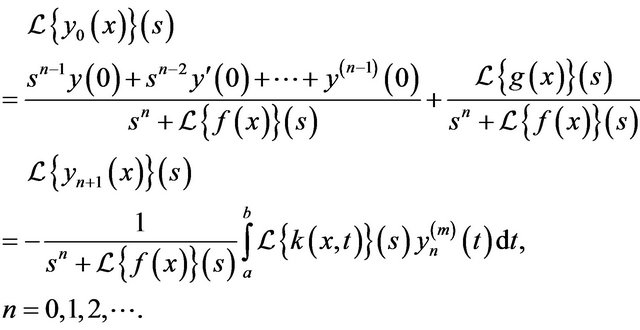 (2.3)
(2.3)
A necessary condition for (2.3) to comply is that

Applying the inverse Laplace transform to both sides of the first part of (2.3) gives , and using the recursive relation (2.3) gives the components of
 . We then define the
  -terms approximant to the solution
 by
by  with
with
 . In this paper, the obtained series solution converges to the exact solution.
2.1. A Test of Convergence
The convergence of the method is established by Theorem 3.1 in [9]. In fact, on each interval the inequality  is required to hold for
 , where
  is a constant and
  is the maximum order of the approximant used in the computation. Of course, this is only a necessary condition for convergence, because it would be necessary to compute
  for every
  in order to conclude that the series is convergent.
2.2. Definition
Let  be the successive approximations to the solution
  of a problem. If the positive constants
 ,
,  exist such that

then we call  the (estimated) Local Order of Convergence (EOC) at the point
 . The constant
  is called Convergence Factor at
 .
.
3. Applications
In this section, the CLT-ADM for solving nth-order integro-differential equations is illustrated in the three examples given below. To show the high accuracy of the solution results from applying the present method to our problem (2.1) compared with the exact solution, the maximum error is defined as:

where  represents the number of iterations. Moreover, we give a comparison among the CLT-ADM, Homotopy perturbation method (HPM) [1] and the variational iteration method (VIM) [2]. The computations associated with the examples were performed using Maple 13 package.
Example 1
Solve the second-order integro-differential equation by using the CLT-ADM [1,2]:
 (3.1)
(3.1)
As mentioned above, taking Laplace transform of both sides of (3.1) gives

so that
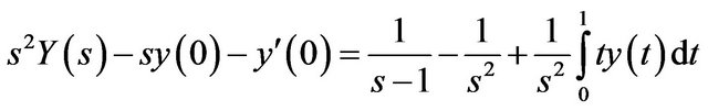
or equivalently

where . Substituting the series assumption for
  as given above in (1.2), and using the recursive relation (2.3) we obtain
 (3.2)
(3.2)
Taking the inverse Laplace transform of both sides of the first part of (3.2) gives , and using the recursive relation (3.2) gives

Thus the series solution is given by

that converges to the exact solution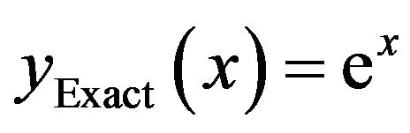 . In Table 1, the maximum errors and the EOC are presented for
 . Comparing it with the HPM and VIM results given in [1,2], we notice that the result obtained by the present method is very superior (lower error combined with less number of iterations) to that obtained by HPM and VIM. From Table 1, it can be deduced that, the error decreased monotically with the increment of the integer
 .
.
Example 2
Solve the third-order integro-differential equation by using the CLT-ADM [1,2]:
 (3.3)
(3.3)
As early mentioned, taking Laplace transform of both sides of (3.3) gives

so that

or equivalently

where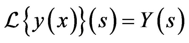 . Substituting the series assumption for
  as given above in (1.2), and using the recursive relation (2.3) we obtain
 (3.4)
(3.4)
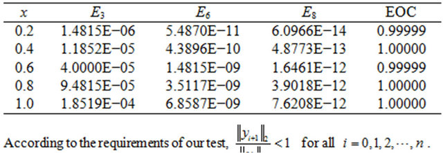
Table 1. Maximum error and EOC for Example 1.
Taking the inverse Laplace transform of both sides of the first part of (3.4) gives , and using the recursive relation (3.4) gives

The series solution is therefore given by

that converges to the exact solution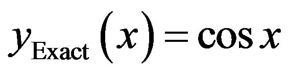 . In Table 2, the maximum errors and the EOC are shown for
 . Comparing it with the HPM and VIM results given in [1,2], we notice that the result obtained by the present method is very superior (lower error combined with less number of iterations) to that obtained by HPM and VIM. From Table 2, it can be concluded that, the error decreased monotically with the increment of the integer
 .
.
Example 3
Solve the eighth-order integro-differential equation by using the CLT-ADM [1,2]:
 (3.5)
(3.5)
As previously mentioned, taking Laplace transform of both sides of (3.5) gives

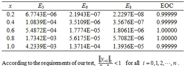
Table 2. Maximum error and EOC for Example 2.
so that

or equivalently

where . Substituting the series assumption for
  as given above in (1.2), and using the recursive relation (2.3) we obtain
 (3.6)
(3.6)

Taking the inverse Laplace transform of both sides of the first part of (3.6) gives , and using the recursive relation (3.6) gives

and so on for other components. Consequently, the series solution is given by

Table 3. Maximum error and EOC for Example 3.

that converges to the exact solution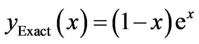 . In Table 3, the maximum errors and the EOC are given for
 . Comparing it with the VIM results given in [2], we realize that the result obtained by the present method is very superior (lower error combined with less number of iterations) to that obtained by VIM. From Table 3, it can be deduced that, the error decreased monotically with the increment of the integer
 .
.
4. Conclusion
The CLT-ADM has been applied for solving nth-order integro-differential equations. Comparison of the results obtained by the present method with that obtained by HPM and VIM reveals that the present method is superior because of the lower error and less number of needed iteration. It has been shown that error is monotically reduced with the increment of the integer n.
5. Acknowledgements
We would like to thank the referees for their careful review of our manuscript.