Semi-Automatic Modeling Technique of Torque Converter Flow Passage ()
1. Introduction
Semi-automatic modeling refers to programming and, with the help of a computer, to directly generating the model for numerical simulation. In the research and design of the torque converter, the flow field numerical simulation has become an indispensable procedure. Many scholars have done a lot of work in numerical simulation (Masatoshi Yamada et al. [1], R. R. By et al. [2], Hyuk Jae Chang et al. [3], Pradeep Attibele et al. [4], Marco Cigarini et al. [5], Zhao Dingxuan et al. [6], Yan Peng et al. [7], Tian Hua et al. [8], H. Schulz et al. [9], Won Sik Lim et al. [10]). In general, the flow passage model of a converter wheel is a hexahedron which includes 6 curved surfaces. For such a complex shape, modeling is a challenging task. On the one hand, the existing modeling methods are uneasy to ensure the accuracy of the model (Won Sik Lim et al. [11]). Obviously, the accuracy of Mode not only affects the accuracy of solution, but also affects the convergence of the iterative process. On the other hand, the existing modeling methods also spend too much time. Even if some modeling software is used for modeling in a human-machine-dialogue manner, the modeling is also a very time-consuming work.
Fluent is the most widely used CFD software, and its pre-processing software Gambit can be used to create a two-dimensional or three-dimensional model. However, for such a complex model of converter wheel passage, it is not very effective for Gambit to be used for modeling. Therefore, some scholars completed modeling with the help of the other software in a human-machine-dialogue manner. Some examples state that the communication between Gambit and the other modeling software is successful. On the other hand, References [12] and [13] established an analytic research and design system of torque converter which laid the mathematic foundations for the semi-automatic modeling. If a program code is developed which is used for the design and modeling of a torque converter, and an interface between high-level programming language and the modeling software is created, the semi-automatic modeling technique is feasible.
The flow passage model of a torque converter wheel includes four revolution surfaces (inner wall surface, outer wall surface, entrance surface and exit surface) and two freeform surfaces (point-based surfaces) which are blade external surfaces. Therefore, the flow passage model of torque converter can be considered as a revolution entity sliced by two curved surfaces.
2. Approximation of the Meridional Streamlines of Inner and Outer Wall
In order to facilitate modeling, the meridional streamlines of inner and outer wall can be approximated with circular arcs. In general, according to evaluation indexes, there are three kinds of curve approximation methods. The first method is square approximation. The advantage of square approximation is that each coefficient of the fitted equation can directly be obtained by solving linear equations. The disadvantage is that the deviation of some points may be substantially large. The second method is that the residual serves as the objective function and is mathematically called optimum approximation or uniform approximation. The optimum approximation makes the maximum error as small as possible. Therefore, the optimum approximation is more reasonable. However, in fact it is very difficult to directly obtain coefficients of the fitted equation. In addition, the relative error can serve as the objective function, which can be called relative approximation. The relative approximation can give a quantitative feeling, but it is difficult to directly find the coefficients of the fitted equation as well. For a converter wheel, the starting and ending point parameters of meridional streamlines serve as original parameters and the parameter errors at the two points should not be allowed. After the design conditions of torque converter is taken into account, a new approximation method, condition optimum arc approximation, is put forward. The basic idea of the approximation is as follows: first, construct a circular arc by using three points, and then optimize it by adjusting the coordinates of the intermediate point. In this manner, the parameters of the arc equation can be obtained.
For any converter wheel, according to the [12], take on , thus, the meridional streamline equation of inner wall is
 (1)
(1)
The x-coordinate at a point located on the meridional streamline of inner wall is
 (2)
(2)
The y-coordinate at a point located on the meridional streamline of inner wall is
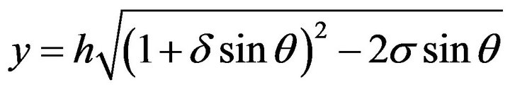 (3)
(3)
In order to approximate the meridional streamline of the inner wall, the polar angle  needs to be discretized. Take on
 , where
  is the polar angle at the starting point and located on the meridional streamline of the inner wall, while
  is the polar angle at the ending point and located on the meridional streamline of the inner wall.
By using (2) and (3), the discrete point x-coordinates  and y-coordinates
  can be obtained.
Assume that the circular arc equation takes the form of
 (4)
(4)
The condition optimum arc approximation of the meridional streamline of the inner wall can be described as follows:
Under the condition of  and
and , the radius residual approaches its minimum, that is
 (5)
(5)
where  and r are used to represent the x-coordinate of arc center, y-coordinate of arc center and arc radius, respectively.
  and
and  are the x-coordinate and y-coordinate of the first discrete point, while
  and
and  are the x-coordinate and y-coordinate of the last discrete point.
Because there are both positive and negative bias, and there are always

Consequently, Equation (5) can be rewritten as
 (6)
(6)
To obtain the arc equation parameters  and r, the starting point
 , the ending point
  and the intermediate point
  can be used to construct an arc (
 , rounding). Substituting the coordinates of the three points into (4), we have
 (7)
(7)
The first formula of (7) is used to subtract the second and the third formula of (7) respectively, and then they are rearranged. We can obtain
 (8)
(8)
where
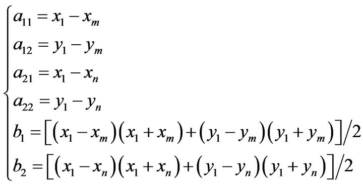 (9)
(9)
Solving (8) by using Cramer’s Rule, the central coordinates and radius of the circular arc are
 (10)
(10)
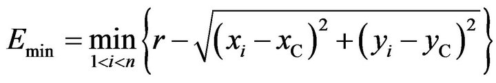
The maximum error of the arc approximation is
 (11)
(11)
The minimum error of the arc approximation is
 (12)
(12)
If , the arc equation determined by the above parameters is the condition optimum arc approximation of the meridional streamline of inner wall. Otherwise, the above parameters need to be corrected by optimization.
If the vector from arc center  to intermediate point
  is expressed as
 , the correction values of the intermediate point coordinates take the form of
 (13)
(13)
where  is a correction factor less than 1 and can take on 0.7 generally.
Substitute  for
for  and substitute
  for
for , iterating by using (9)-(13). After several iteration steps, the parameters of the arc equation hardly vary. Thus, the condition optimum approximation arc parameters of the meridional streamline of inner wall can be obtained.
Similarly, the condition optimum approximation arc parameters of the meridional streamline of outer wall can be obtained as well.
3. Calculation of Slice Surface
Slice surfaces are the two lateral surfaces of flow passage. One lateral surface is the pressure surface of a blade, while another lateral surface is the suction surface of the adjacent blade.
3.1. Basic Idea of Slice Surface Calculation
From [12] and [13], it can be found that the central stream surface (or blade camber surface) cannot be expressed as a rectangular coordinate equation. Therefore, it is difficult to directly derive the equation of blade surface or the equation of flow passage lateral surface. A feasible option is to calculate the coordinates of discrete points by numerical method.
Discrete parameter  and polar angle
 . In other words, take on
 , and
, and .
.
In order to calculate the point coordinates on blade surfaces, an imaginary blade is arranged just in the central stream surface of flow passage. The relation among flow passage central stream surface, the surfaces of the imaginary blade and the flow passage lateral surfaces is shown in Figure 1.
First, calculate the coordinates of Point P located on central stream surface of the flow passage. Then draw a

Figure 1. Relation among passage lateral surface, imaginary blade surfaces and flow passage central stream surface.
normal line of the central stream surface passing through point P. In this manner, intersection Points A and B are obtained. They are located on two external surfaces of the imaginary blade, respectively. Finally, rotate the Point A and B a half of flow passage angle  around x-axis in different directions, respectively. Points C and D can be obtained. The two points are located on the lateral surfaces of the flow passage.
According to [12], the coordinate calculation formula of the flow passage central stream surface is
 (14)
(14)
where

For the given  and
and , the coordinates of any discrete point on the flow passage central stream surface can be calculated.
3.2. Approximation of Central Stream Surface
As the equation of central stream surface is substantially complex, it is difficult to obtain the normal equation of the central stream surface. Therefore, a quadratic surface is used to approximate the central stream surface. For a given point , the point and its surrounding 8 points are used to construct a quadric surface. Assume that the equation of the quadric surface takes the form of
 (15)
(15)
where  and
and  are all coefficients to be determined.
The constant item of (15) takes on 1000 rather than 1 so as to avoid too small coefficients.
Inserting the coordinates of the above 9 points into (15), we have
 (16)
(16)
where


It should be noteworthy that the existence and uniqueness of the equation solution need to be investigated before solving (16). According to the linear algebra theory, the necessary and sufficient condition for the existence and uniqueness of solution is that the coefficient matrix of the equation is a non-singular matrix, or . The solution error of the simultaneous equations is closely related with the ill-posed problem of the equation. The condition number of equation needs to be used to determine if an equation is ill-posed (Xi Meicheng [14]). Obviously, it is difficult to prove whether the matrix is a non-singular matrix or not in advance. Similarly, it is uneasy to determine if an equation is ill-posed in advance. However, for the given practical engineering example, it should be seen that the central stream surface is a smooth surface. No dramatic curvature change occurs and there is no singularity either. It should be said that the existence and uniqueness of the equation solution is undoubted.
There are many methods of solving linear equations. Column pivot Gauss-Jordan elimination method is used to solve (16). The ill-posed problem taken into account, some pre-processing measures are taken and doubleprecision format data are used for program design. By solving the linear equations, each coefficient of (15) can be obtained.
3.3. Numerical Calculation of Passage Lateral Surface
Let

Take partial derivatives of the above expression, there resulting

The normal vector of the quadric surface passing through point  is
is
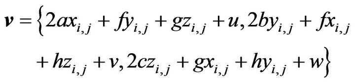 (17)
(17)
With the normal vector of the quadric surface, assume that the thickness of the blade is 2t. For a punched blade ; for a casted blade
 . The coordinates of Point A shown in Figure 1 are
 (18)
(18)
The coordinates of point B are
 (19)
(19)
With coordinates of Point A and B, by using the coordinate rotation formula, coordinates of Point C are
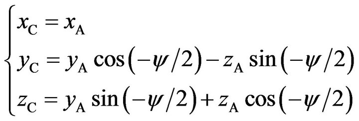 (20)
(20)
Coordinates of Point D are
 (21)
(21)
Coordinates of Points C and D are stored in file Converter.txt. With coordinates of Points C and D, the offset angles corresponding to the above two points are
 (22)
(22)
It can be inferred that offset angle  and
and  are the function of parameter
  and
and , naturally varying with
  and
and . By means of the program, the maximum offset angle
  and minimum offset angle
  of the flow passage can be obtained conveniently. They are
 (23)
(23)
4. Generation of Flow Passage Mode
4.1. Automatic Generation of Revolution Entity
If meridional streamlines of inner and outer wall of torque converter are approximated with arcs, the torus of each converter wheel consists of two arcs (inner and outer wall) and two straight line segments (entrance and exit). Pump torus is shown in Figure 2.
Coordinates of arc endpoints, center coordinates of inner and outer arc, and arc radii have been calculated. The central angle of the outer arc (from Point 3 to 4) is
 (24)
(24)
By using high-level language programming for the above calculation, the parameters of all graphic entities (straight line segments and circular arcs) can be obtained. With the graphic entity parameters, the torus of each converter wheel can be generated automatically by using a drawing program.
In order to generate a three-dimensional revolution entity with the above torus, the “revolve” command of Auto CAD needs to be applied. The command need specify a revolution angle. Theoretically, the revolution angle should be equal to the difference between the maximum offset angle  and minimum offset angle
  of the flow passage. In fact, after considering 10˚ margin and rounding, the revolution angle takes on
 .
.
The “revolve” command of Auto CAD is prescribed to revolve an angle from 0˚ to . In general, the revolution angle of model is often not in the range. Therefore, it is necessary to adjust the space position of the revolution

Figure 2. Pump torus of hydrodynamic torque converter.
entity. Thus, the “rotate3d” command of Auto CAD needs to be applied. Similarly, after considering 5˚ margin and rounding, the rotation angle of the “rotate3d” command takes on .
.
The developed high-level language program can output a file converter.lsp which is a drawing program and includes various drawing commands. By using Auto CAD, the three-dimensional revolution entity can be generated automatically and stored in file RevolutionEntity.sat. Next, with the help of Solidworks, transform the file into RevolutionEntity.sldprt file.
4.2. Generation of Slice Surfaces
Run Solidworks, open the file Converter.txt, read in the point cloud data, and then the points on the slice surfaces of the flow passage will appear in Solidworks graphic window, as shown in Figure 3.
In order to transform these discrete points into smooth surfaces, the ScanTO3D Wizard tool can be used to accomplish this function. The generated slice surfaces are shown in Figure 4.
4.3. Inserting Revolution Entity
In the drop-down menu of Solidworks, select “Insert Part” command, select the RevolutionEntity.sldprt. Thus, the revolution entity is inserted into the graphic window of SolidWorks, as shown in Figure 5.
4.4. Slicing the Revolution Entity
By using “Insert” command as well as its sub-command, the entity slice is completed. After slicing, the entity is shown in Figure 6.

Figure 3. Discrete points on slice surfaces.

Figure 5. A revolution entity and two slice surfaces.
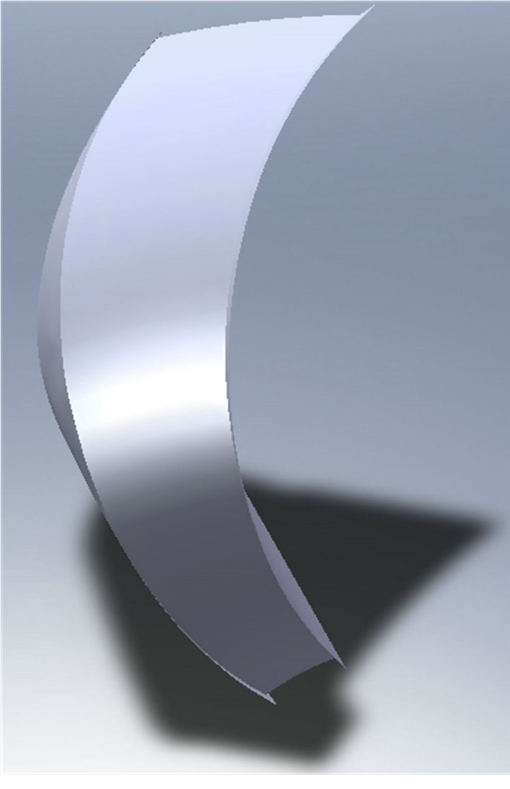
Figure 6. Revolution entity after slicing.
From Figure 6, it can be seen that the two slice surfaces still exist after completing slice operation. This is because Solidworks software was design in history base. The two surfaces cannot be deleted simply. Otherwise the model will be destroyed. The simplest solution is to insert the entity into a part drawing.
Something also needs to be said about the file format used to store the model. Parasolid format can be a correct selection. Enter the file name Converter.x_t, and save the file. At this stage, the model of pump flow passage is shown in Figure 7.
From Figure 7, it can be found that each lateral surface of flow passage model is not a single surface, but consists of a number of small surfaces. Moreover, the number of small surfaces is not fixed.
4.5. Further Process of Flow Passage Model
In order to facilitate the automatic generation of mesh, by using Gambit, these small surfaces of each lateral surface can be merged into a large surface, so as to make the model become a surface hexahedral. After merging surfaces, the model is shown Figure 8.

Figure 7. Pump flow passage model created by using one revolution entity and two slice surfaces.

Figure 8. Pump flow passage model after merging small curved surfaces.
5. Parameterized Program
In order to achieve modeling automation or semi-automation, a parameterized program code is developed. Various design and modeling tasks, such as, design calculation, graphic drawing, file output, etc., are accomplished with the program code. The program’s input and output interface is shown in Figure 9.
From the figure, it can be seen that the program interface includes 10 input parameters and 2 output parameters. After the input parameters are given, click on the Design button. It can be observed the 2 output parameters. If the 2 output parameters are satisfactory, click on the Exit button to end the program. After running, the program will output two important files, Converter.lsp and Converter.txt. The former is used to generate a threedimensional revolution entity, while the later is used to generate two slice surfaces.
Practice has stated that the various design and modeling tasks can be completed within several minutes with the help of the program code.
6. Model Error Analysis
Of the six surfaces of the torque converter flow passage model, entrance surface and exit surface are accurate, while the inner wall surface and the outer wall surface are not very accurate. In addition, the two lateral surface of the flow passage model are not very accurate, either. The errors of the inner surface and the outer wall surface result from the approximation of meridional streamline, while the errors of two lateral surfaces of the flow passage model result from the approximation of central stream surface.
6.1. Meridional Streamline Approxi-Mation Error
As meridional streamlines of inner and outer wall are approximated with circular arcs, which will result in model error. The error can be expressed as the arc radius

Figure 9. Input and output interface of program.
error. With the help of the program code, the absolute error and relative error of arc radius can be obtained directly. As an example, model error of YB355 torque converter is calculated.
For the pump and turbine, the maximum absolute error of inner wall arc radius is 0.19376853 mm, and the maximum relative error is 0.7983%. The maximum absolute error of outer wall arc radius is 0.43897597 mm, and the maximum relative error is 0.7703%.
For the stator, the maximum absolute error of inner wall arc radius is 0.02159697 mm, and the maximum relative error is 0.080558%. The maximum absolute error of outer wall arc radius is 0.1617693 mm, and the maximum relative error is 0.326664%. These data indicate that the condition optimum arc approximation possesses substantially high approximation accuracy and can meet the requirements of engineering practice.
6.2. Central Stream Surface Approxi-Mation Error
As the central stream surface is approximated with a quadratic surface, the node coordinates are accurate, but the other point coordinates are not very accurate. It is very difficult to derive the error formula used for the quadratic surface approximation. A feasible selection is to directly calculate the errors by using numerical method.
First, take on  and
and  . Next, by using (14), theoretical coordinate
  and theoretical revolution radius
  can be obtained. After that, substitute
  and
and  into (15). Finally solve the equation for
 . Thus, approximate coordinates are
  and
and .
.
The absolute error expressions of y-coordinate and z-coordinate are
 (25)
(25)
The relative error expressions of y-coordinate and z-coordinate are
 (26)
(26)
With the help of the program code, the error values can be obtained.
For the pump, the absolute error eymax = 6 × 10⁻⁶ mm and ezmax = 23 × 10−6 mm. The relative error εymax < 10−6% and εzmax < 10−6%.
For the turbine, the absolute error eymax = 6 × 10⁻⁶ mm and ezmax = 52 × 10−6 mm. The relative error εymax < 10−6% and εzmax < 10−6%.
For the stator, the absolute error eymax = 22 × 10−6 mm and ezmax = 44 × 10−6 mm. The relative error εymax < 10−6% and εzmax < 10−6%.
The above data clearly show that the quadric surface approximate is substantially accurate and able to meet the requirements of engineering practice.
7. Conclusions
The modeling technique of torque converter is investigated. The main results of this paper are as follows:
1) The semi-automatic modeling technique of torque converter is put forward and implemented;
2) A new approximation method, condition optimum approximation, is proposed. And, the method was used for the arc approximation of the meridional streamlines of inner and outer wall. In this manner, the problem that the three-dimensional revolution entity is automatically generated is solved;
3) The central stream surface of flow passage is approximated with a quadratic surface. The coordinates of the blade surface points and the flow passage lateral surface points are substantially accurately calculated with numerical method. The problem of automatic generation of slice surface is fairly well solved;
4) The various tasks (design calculation, graphic drawing, file output, etc.) are accomplished with a parameterized program code, achieving semi-automatic modeling of torque converter passage, and greatly reducing the modeling time-consumption;
5) By means of the program code, the errors of flow passage model are calculated and analyzed with numerical method. The error estimation of modeling was solved.
In short, the semi-automatic modeling technique is of engineering application value.
8. Acknowledgements
The authors wish to thank the financial support of Henan Provincial Tackle Key Program of China. In addition, the authors would like to thank Prof. L. Quan, for his help and advice in the research.
Nomenclature
 distance from rotation axis line to the geometric center of design streamline;
 polar angle at a point located on the meridional streamline;
 polar radius at a point located on the meridional streamline;
 constant;
 ;
;
 geometric radius of design streamline;
 arc radius or revolution radius;
 offset arc length;
 one half of blade thichness;
 offset angle;
 arc central angle;
 flow passage angle (
 divided by blade number);
 Cartesian coordinates;
 parameter used to specify blade span direction,
 . For the inner wall
 ; for the outer wall
 ; for the design streamline
 .
.
Subscription
 arc center;
 first discrete point or pump/turbine/stator inlet;
 theoretical value;
 approximation calculation value;
 last discrete point or pump/turbine/stator exit;
 intermediate discrete point.