A New Energy Efficient Data Gathering Approach in Wireless Sensor Networks ()
1. Introduction
Wireless sensor networks are a class of wireless ad-hoc networks. In these networks, sensor nodes collect data from physical environment and after processing sent to the base station (BS1). Thus allow monitoring and control many types of physical parameters. Each sensor node has limited energy and in most applications, replacing energy sources are not possible. So lifetime of sensor nodes is highly dependent on energy stored in their battery. Clustering is a designing method that used for management of wireless sensor networks. In this method, the network is divided into several independent collections that these collections called cluster. So each cluster contains a number of sensor nodes and a cluster head node. Member nodes in a cluster send their data to relative cluster head node. Cluster head node aggregates these data and send to the base station. Therefore, clustering in sensor networks has advantages such as data aggregation support [1], data gathering facilitation [2], organizing a suitable structure for scalable routing [3], and efficient propagation of data in the network [4].
Data gathering in wireless sensor networks is an important operation in these networks and for this purpose many methods have been proposed. The LEACH2 [5] protocol has been considered as a hierarchical basic method. This method is suitable for monitoring applications. Each node periodically senses the information and sends them. In this algorithm, the clustering method has used for data gathering and aggregation. The cluster and cluster head selected randomly, therefore there is no assurance to select the exact improved number and uniform distribution of cluster head throughout the network. Many improvements in LEACH protocol have been presented. LEACH-C3 method [6] is an example of these improvements. In LEACH-C, the forming of clusters is done using a centralized algorithm by the base station in the starting of each period. Base Station uses the received information from nodes for finding the predetermined number of cluster heads and network configuration within the clusters. This information contains position and energy of nodes. Another improvement to this algorithm is the use of estimation. One of these algorithms is LEACHCE4 [7]. In the proposed technique energy level collected from all nodes in two primary periods but not collected in the other periods. Instead, the average energy of initial periods is used. Considering that the energy estimation in this method is not precise, this clustering scheme is not efficient and suitable. There is some proposed clustering methods that ABCP [8] and ABEE [9] and HMM [10,11] are samples of them.
Each sensor node is observer of a physical phenomenon. Also physical phenomenon such as temperature and... continuously change in time. So the information provided by sensor nodes is dependent on each other. Some algorithms that based on not sending of correlated data are considered. The TINA5 [12] algorithm is one of them. In this algorithm the sensor node compares the value of sampled data with previous data, if that be different send it and otherwise goes to sleep mode. The proposed improvement to this algorithm is that sensor node decides to send data with comparing the value of new sample with last reported data [13]. These mentioned algorithms due to error in report, is not suitable. Therefore, a method proposed to increase the accuracy of data reporting. For precise estimation of nodes energy, the base station must be aware of data time correlation. So with existence of data time correlation and using energy estimation of nodes, a method suggested so that the base station can estimate nodes energy precisely. These methods avoid the overhead excess and increase the network lifetime.
The remaining of this article is organized as follows: In Section 2 related works are reviewed. In Section 3 we introduce correlated data algorithm with the energy predicting technique and the hybrid method. analysis of experiments with existing nodes offered in Section 4, and we finally in Section 5 summarize and discuss the scheme.
2. Related Work
2.1. LEACH
One of the most famous hierarchical routing protocols based on clustering, is the LEACH protocol. In this method, each cluster members send their data to cluster head. The cluster head aggregate this data and send to the BS. So the communication cost is reduced. Figure 1 describes this concept:
The operation of cluster forming and data transmission in LEACH is done in two phases that these phases shown in Figures 2 and 3:
Setup phase is the stage of forming cluster and cluster head. At this stage, cluster and cluster head randomly selected. After forming the cluster, cluster head propagate TDMA6 scheduler to specify the data transfer time to member nodes. Then the steady-state phase started. In the steady-state phase, each member node in cluster send data to the cluster head only in its time slot and at the rest of time pieces for energy conservation goes to sleep mode.
In this method, the cluster head consumes more energy for receiving, processing and directly sending this data to the BS node. So for increasing the life time of the network it is necessary to replace role of cluster head between network nodes. Many improvements over the LEACH method have been provided that in these improvements firstly, as far as possible the best clustering and cluster head selection is done, secondly possible as possible overhead of the protocol is to be reduced. LEACHC method is an example of these improvements.
2.2. LEACH-C
In LEACH-C, clusters forming in the beginning of every period are done, using the centralized algorithm by the base station. The base station uses received information from nodes that includes energy and node status, uses

Figure 1. A sensor network with clustering.
this information during the setup phase for finding predetermined number of cluster heads and network configuration within the clusters. Next classification of nodes in the clusters is done to minimize energy consumption in order to transfer their data to the related cluster head. Results show that LEACH-C overall performance is better than LEACH because of the optimal forming of clusters by the base station. In addition, the number of cluster heads in each period of LEACH-C is equal to the expected optimal value. While in LEACH the number of cluster heads varies in different periods because of lack of global coordination.
As in LEACH-C at the beginning of every period energy of nodes must be sent to BS, therefore nodes early discharged and the network lifetime reduces. Another improvement on this algorithm is the use of energy estimation. The LEACH-CE method is an example of these methods.
2.3. LEACH-CE
In the LEACH-CE method, the energy level of all nodes collected only in two primary periods and not be collected in other periods. Instead because of knowing information about energy level of nodes, we can calculate energy consumption average for each node by using information of two primary periods. This means that reducing calculated energy level from the energy level of node, causes predicting current energy level of node. The problem of this algorithm is that firstly energy estimation is not done precisely and secondly if nodes have correlated data, while not sending correlated data means that previous data is valid, so this plan of clustering is not suitable and efficient.
2.4. TINA
Phenomenon that observed by sensor nodes, continually change in time. Therefore information received by the nodes is correlated on each other. These cases for physical phenomena that are continuous or repetitive, or in an application that the accuracy is not too important, or in a network that node density in a region is high, have seen more. There are two types of data correlation: 1) spatial correlation; 2) Time correlation.
In the spatial correlation, aggregation is done within the network by cluster heads. This is one of the proposed methods to reduce energy consumption. So the nodes that have correlated data send them to cluster head and cluster head after aggregating these data send to the base station. This causes to prevent waste of energy. This method has been implemented in LEACH protocol.
But in the time correlation, each node can have correlated data in successive times. Mohamed and Sharaf proposed the TINA algorithm. The main idea of TINA algorithm was that the sensor nodes send their data only when this data differ with previous data otherwise goes to sleep mode. This algorithm has a reporting error. There is an improvement to this algorithm that presented below.
2.5. Improvement of TINA
In this method, the sensor node decides to send data by comparing the value of newly sampled data with last reported data. However, sensor nodes maintain last reported data. For better understanding, we describe this section with an example. Suppose that a given sensor node that received data are 1.0, 0.95, 1.05, 0.95, 1.05 respectively. A threshold has been considered that data changing to this threshold is not important. The value of this threshold considered equal to 10%. First given data that is equal to 1.0 successfully sent and in the next period 0.95, will not be sent when: 
Otherwise that will be sent. In the third stage 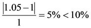 that will not sent and in the fourth stage
  that will not sent. This method is suitable when phenomenon changes have not a lot of swing or any special event in the network is done. But as mentioned previously most of phenomenon change continuously with time. So most of data are in ascending or descending mode in the time slices. Or in an application such as temperature for example in a certain time slot occurs a specific event. So the proposed methods have errors and are not suitable. We offer a method to improve this algorithm and prevent the waste of energy. In addition, the problem of data time correlation is not considered in proposed protocols. Therefore, we will check the time correlation of data in the proposed algorithms.
3. The Proposed Method
3.1. Presentation of Methods
Three ideas are proposed here: 1) the data time correlation; 2) Energy estimation model of nodes and 3) the hybrid method.
In the data time correlation algorithm, Time Series Forecasting method (TSF7) used to decide sending or not sending of data. Then in time t in the beginning of each period, base station send percentage of error e(t) to all nodes. First data sensed by node and sent. Second and third and fourth data sent based on the improved TINA algorithm. Then the node runs time series function to determine the value of prediction of trend line model, to create trend model. In the next times the sensed data compared with predicted value of trend model, if the difference between these two values exceeds a threshold value, data sent to the given node and the node recalculate prediction function of trend model to update the trend line. Otherwise, the sensor node does not send the sensed data with this insurance that sensed data placed in accuracy range of data. So only some data have to be sent that are very different from the trend line model. This help to prevent energy loss.
We call the node energy prediction model LEACHCEC8 and describe as follow. For doing the best clustering, that is needed to know energy of the nodes. The estimation method is a method that has low cost and is suitable. We also use the energy estimation method. For this, we divided LEACH-C protocol to three phases. Topology building phase, setup-state and steady-state. In the first phase nodes send their position to the BS. Then BS creates network topology based on these positions. Once the topology was formed in the base station, base station node calculates the distance of nodes to each other. The BS calculates the amount of energy used in each node in the setup-phase, using a simple mathematical model. Then deduct this amount from primary energy and calculates its remaining energy. Finally do the clustering and goes to the steady-state phase. In this phase for each node, the data time correlated algorithm applied according to the following method.
BS node should be informed of data time correlation in nodes to estimate precisely energy of them. Therefore cluster head create a table that containing list of all members of the cluster. Cluster head registers every node in to the table that have correlated data and do not sent in certain times. In the end of each period, cluster head sends this table with collected data to the base station. This table contains nodes ID and number of times that these nodes not sent data. Base station uses this information for clustering decisions in centralized methods. Ultimately that cause to energy estimation in centralized methods is more carefully while the best clustering is created and the network lifetime increases. So in total lifetime of the network, first phase has done once but setup and steady-state phases done as in LEACH-C.
3.2. Process of Proposed Methods
3.2.1. Linear Prediction Method Using Time Series
Linear prediction method is a powerful technique to predict time series in an environment changing with time. Suppose that you want to contact an independent variable x and a dependent variable y to specify. If we assume that the true relationship between these variables in a straight line and the value observed for each value of y for every given x is a random variable then we can wrote:
 (1)
(1)
where in this equation  is the width from the origin and
  is the slope of the line that is unidentified fixed values. Observed value y can be described with the following equation where the error ε created because of not conforming real value to the amount of predicted value.
 (2)
(2)
This pattern is usually named a simple linear regression model. Because that has only one independent variable so that the x independent variables called prediction variable and y called the response variable. Prediction and response variables x and y can be time series in which case we have a time series regression pattern.
There are several methods to estimate unknown parameters ,
,  in equation (2) that can be used. One method that a lot used is the least square error method in which the
 ,
,  estimates obtained from minimizing sum of squares errors or remaining’s. Suppose we have n observations of (x1, y1), (x2, y2) ··· (xn, yn). A model that is based on these observations is written as follows:
 (3)
(3)
And the total square error is as the follow:
 (4)
(4)
So the total square error is simply the total squares of deviations observed yi and . The estimated values of
  and
and  that we call them
  and
and  that achieved using the least squares method by minimizing
  toward
  and
and  so we can write:


This system of equations called least squares line normal equations system that simplified as the following:


By solving this system  and
and  estimates or on the other hand
  and
and  obtained and so:


where  and
and . So the fitted simple linear regression model is as follows:
For each value of the predicted variable x we can obtain corresponding value predicted response from this equation. The fitted values of  corresponding to observed values
  for every i = 1, 2, ···, n is the following:
The difference between ith given fitted value to an observed yi value called a residue so that:
 (5)
(5)
If the fitted model regression for data is appropriate, in this case remains do not follow of appropriate form. There is no clear pattern for the remains.
This method stated by equation (11) that is a recursive method [9]:
Linear prediction method is a powerful technique for predicting time series in a time-varying environment. This method is expressed in equation (6) and is a recursive method [9,10]:
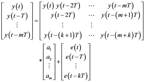
 (6)
(6)
Estimated value at time t as a linear function of previous values in the times “t − T, t − 2T, ···, t − mT” has been produced is obtained. In Equation (1) a1, a2, ···, am are the linear prediction coefficients, “m” is the model degree, “T” is the sampling time, y(t + T) is the next observation estimation and y(t), y(t − T), …, y(t − mT) are the present and past observations. The prediction error which is the difference between the predicted and the real values (Equation (7)) must be minimized.
 (7)
(7)
In order to estimate the coefficients of linear prediction model we use the least squares error method and rewrite Equation (6) with considering modeling error in equation (8):
 (8)
(8)
The error e(t) is generated because of not adopting the linear prediction model to the real value. So to find the coefficients, a1, a2, ···, am in Equation (8) we use the sum least squares error and set of linear functions. Presented in Equation (9).
 (9)
(9)
 (10)
(10)
Elements in the matrix A are the coefficients which can be found by least squares error method (11):
 (11)
(11)
In Equation (11), φT, is the transpose of the matrix φ, and (φTφ) is the inverse of matrix. In practice:
• If m is chosen larger than is required (i.e. over-estimation of the model order), Equation (11), cannot be solved for any unique set of coefficients, because of some columns in the matrix φ, are not independent of each other. Hence φTφ would be unique and will not have inverse. This means that the system of equations in Equation (8) will have an infinite number of answers for the coefficients. Geometrically speaking, it is like fitting an infinite number of lines to a single point which is not the preferred case.
• If m is chosen less than the required value, the number of independent equations would be more than the number of unknown variables (a1 – am). Such a system of equations has to be solved for the best approximation of coefficients. The best approximation for coefficients (a1 – am) is the use of the least squares error method.
Obviously, that is how much precision, the number of the data sent will increase and vice versa.
3.2.2. The Algorithm Used to Estimate the Energy by Transferring Topology to the Base Station
As previously mentioned, LEACH-C protocol divided to three phases: topology building phase, setup-state and steady-state and this algorithm is proposed as following. These three phases is called LEACH-CEC.
a) Topology building phase
1) Start of network.
2) Base station receives position of all nodes that contain x and y.
3) Base station calculates distance of all nodes with each other’s using the following Formula (12):
 (12)
(12)
4) End of phase.
b) Setup-state phase
5) If clustering has changed 5.1) BS calculate energy consumption per node using the Formulae (13) and (14):
 (13)
(13)
and
 (14)
(14)
And after computing, place the sum of two variables in to the .
.
5.2) Base station calculates remaining energy (ER) of each node using the Formula (15).
 (15)
(15)
5.3) BS audit the information received from CHs, if the nodes name with the number of duplicate data is there, considered in terms of computing nodes remaining energy.
5.4) If  the node is dead.
5.5) Otherwise the node is alive and participates in Clustering.
6) Clustering is formed.
 : The amount of consumed energy by node i in time t.
c) Steady-state phase(Hybrid method)
7) If node n is a cluster head.
7.1) Cluster head creates a table containing node name and the number of correlated data.
7.2) Cluster head collects data from the members of the cluster.
7.3) If the cluster head has not received data from its member node, registers name of that node in the table and a unit to be added to the number of correlated data. Cluster head sends the table with correlated data to the base station.
8) Otherwise, that is a member node.
8.1) If the node is in turn on then the node runs correlated data algorithm in figure 4.
8.2) Otherwise goes to sleep mode.

Figure 4. Algorithm of not sending correlated data using TSF.
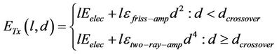
 : Strengthening the energy to transferring 1 bit data in distance d.
 : Radio energy of amplifier.
 : Radio energy of amplifier.
d: distance between receiver and sender l: length of data package.
Table 1 should be created by the cluster head in the steady-state phase. To explain this part, consider a cluster with node numbers 2, 3, 5, 6, 7, 14, and 15 are chosen. Assume that the node 7 is cluster head and the rest is member nodes. If nodes 2 and 5 respectively, each have 2 and 1 correlated data, node 7 as cluster head must create Table 1. This table must be dynamic and at the end of each period must be sent with correlated data.